9 From Text to Data
In most social science applications of text as data, we are trying to make an inference about a latent variable. This is something that we cannot observe directly but that we can make inferences about from things we can observe. For example, we cannot directly observe someone’s ideological position on a spectrum. But we might be able to infer it from seeing—relative to other people—how they respond when asked about specific issues, or who they donate money too, or how warmly they feel about certain politicians.
In this section though, we won’t observe numerical variables, or at least not initially. Instead the things we can observe are the words spoken, the passages written, the issues debated or whatever. There are three type of entities about which we might want to make an inference:
the author: we might want to know how voters of Senators feel about certain issues.
the document: we might want to know whether a given treaty is fair or not, or whether a given bill in Congress is about the economy or not.
both, that is the document and author: we might want to know how presidential speeches change over time, perhaps in response to new issues on the agenda and/or new personalities of the president.
A term you will often here in text work is metadata—it means “data about data”. For example, the author, date of writing and program used to produce a letter to someone might be meta-data of interest, separate to the words themseles.
In any case, we will need to take things that are not numbers—like words—and convert them to numbers such that we can operate on them with the data science tools we’ve been learning about. The very general name for this operation is feature selection or feature representation. In a sense, we have been doing it all along. For instance, we have coded “cigarette tax” as the amount charged per packet, but we could have represented that idea in other ways, and they would have different strengths and weaknesses. A similar logic will apply now.
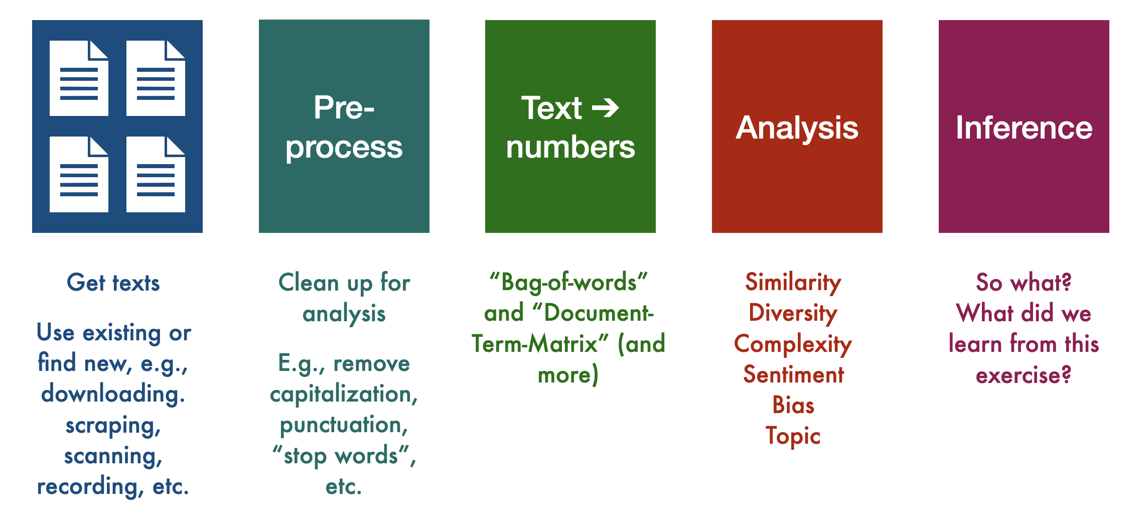
As a high-level overview, here is what will do:
9.1 Useful vocabulary
We will shortly work through a real (albeit simple) example from start to finish to more closely inspect each step. Before we do that, however, we will also need some vocabulary:
9.1.1 Corpus
The corpus is a a collection of documents (plural: corpora). So, the corpus is made up of the documents within it, but note that these may be a sample of the total population of documents available. We sample for reasons of time, resources, or (legal) necessity. For example, you might be able to obtain, say \(\sim 1\)% of all tweets from \(\mathbb{X}\) (formerly known as Twitter) on a given day. You might like to have a larger sample, but they would be prohibitively expensive to store and work with.
In social science, you will hear authors claiming to have universe of cases in their corpus: all press releases, all treaties, all debate speeches and so on. As we have hinted at before, you still need to think about sampling error (noise). This is because there exists a superpopulation of populations from which the universe you observed came from.
As usual, random error (so, noise) may not be the only concern. We want to corpus to representative in some well-defined sense for inferences to be meaningful. For example, if you want to understand how politicians privately feel about some White House policy, their public statements—even in great number—may not be a good source for making inferences (what could we gather instead?).
9.1.2 Document
Often, exactly what constitutes a document is obvious, but sometimes it’s not. For example, if I wanted to study how the New York Times covered the Biden administration, my corpus might be all “NYT articles between January 20, 2021 and January 20, 2025 that contain the word”Biden” at least once. My documents would likely be each article in our corpus. But I could also think of a document as being everything by a particular journalist on the subject. Or a document might be the specific paragraph that mentioned “Biden”.
This can get even more complicated in the case of non-traditional sources like social media. For example, if we were doing an analysis of the sentiment of Twitter users towards Elon Musk after his takeover of Twitter, we might have a corpus that includes a certain number of tweets with the words “Elon” or “Musk” from perhaps the first month of his takeover as well as from the month prior his takeover. In this case, our documents would each be one tweet. But you could also imagine a document being everything by the same author in a multiple tweet thread, or everything the original poster wrote, plus all the replies and quote tweets.
9.2 Reducing Complexity
Language is extraordinarily complex, and involves great subtlety and nuanced interpretation. Consider for an example, the following sentence:
I wouldn’t have been shocked if the chair didn’t show up, given how things have been going on the floor
There are tricky conditionals and double-negatives, and “chair” and “floor” means something very specific. Ultimately the speaker is making a simple point, though. Here’s another one (from the NYT)
The nonpartisan Congressional Budget Office said Wednesday that the broad Republican bill to cut taxes and slash some federal programs would add $2.4 trillion to the already soaring national debt over the next decade, in an analysis that was all but certain to inflame concerns that President Trump’s domestic agenda would lead to excessive government borrowing.
It long, with multiple clauses, and needs a great of attention to follow. These sorts of cases might lead one to believe that text-as-data approaches struggle to represent such sentences exactly in all their nuanced glory. That’s true, but it often doesn’t matter. That is, for many (not all!) applications, we find that we can do very well by simplifying. By this we mean that we can represent documents as straightforward very stripped-down mathematical objects. This makes the modeling problem much more tractable.
By “do very well”, we mean that much more complicated representations add almost nothing to the quality of our inferences or our ability to predict outcomes. Of course, how you should simplify language is dependent on the particular task at hand and there is no “one best way” to from texts to data. But here are the most common steps in basic text-as-data work:
- Collect raw text in machine readable/electronic form. Decide what constitutes a document.
- Strip away ‘superfluous’ material: HTML tags, capitalization, punctuation, stop words etc.
- Cut document up into useful elementary pieces: tokenization.
- Add descriptive annotations that preserve context: tagging.
- Map tokens back to common form: lemmatization, stemming.
- Operate/model.
We call steps 2 through 5 “preprocessing” and, as we say, doing this will make our lives much easier with not too much cost. Here are some more details:
9.2.1 Cleaning and standardization
Depending on our research goals, we will likely want to do some kind of cleaning and standardization of our data. This often requires making decisions about:
- Stop words: commonly used words, such as “the”, “and”, “of”, etc., that we may want to exclude from our analysis. The idea is that there are a larger number of such words, but they don’t add much to our basic understanding of a text. For example, here’s our NYT sentence without “stops”
Nonpartisan Congressional Budget Office said Wednesday broad Republican bill cut taxes slash federal programs add $2.4 trillion soaring national debt next decade, analysis certain inflame concerns President Trump’s domestic agenda lead excessive government borrowing.
The lists of such terms are standardized, but we can add to them if we need to.
- Punctuation & capitalization: if we simply cut up documents by the presence of whitespace, this means that, for example, the words
run,Run, andrun., andrun, would all be stored as unique types. This might be useful for us, but more than likely it is a distraction and unnecessary complication if what we really want to understand is how often the word run is used. Thus, we may want to remove capitalization and punctuation from our text.
Here’s an example sentence from Federalist 1:
The subject speaks its own importance; comprehending in its consequences nothing less than the existence of the UNION, the safety and welfare of the parts of which it is composed, the fate of an empire in many respects the most interesting in the world.
It seems plausible that “UNION” (somewhat arbitrarily uppercased) is the same entity as “Union” used elsewhere and the commas don’t add that much to our overall understanding. So we can lower-case everything, and we can delete punctuation to produce something where the original meaning is essentially completely intact:
the subject speaks its own importance comprehending in its consequences nothing less than the existence of the union the safety and welfare of the parts of which it is composed the fate of an empire in many respects the most interesting in the world
In some cases we might really want to include punctuation—for example if the presence of ! or ? will likely help you better understand the sentiment of your customers or voters. You also might want to retain capitalization if your data includes a lot of proper nouns that, without capitalization, might be lost as such. For example, if we want to understand sentiments about the company “Apple”, we almost certainly would not want to lowercase it, lest we accidentally collect sentiments around fruit.
9.2.2 Tokenizing
We need to chop up each document into units that the computer can make sense of (this is the simplest version; there are techniques where we chop text into sentences, paragraphs, or not at all, and while that can provide more accurate analyses (though not necessarily), it quickly becomes very computationally intensive). By “make sense of” we will mostly mean “count”, but we’ll come back to that.
While we are dealing with terminology, not the following:
- Token: a sequence of characters in a document that are grouped together as a useful unit; e.g., a word or number, like “American” or “1776”. In English, this is often whitespace-based; i.e., we say a token ends when there is a space between letters. This is not always perfect, but it’s a simple and reasonably effective start.
- Type: the number of unique tokens in a document (so, the number of different words in a doc). For example the sentence “Dog eat dog world” has four tokens (dog, dog, eat, world), but three types (dog, eat, world).
- Term: this is a type that is part of the system’s ‘dictionary’ (i.e. what the machine recognizes as a type to be counted). It might not be a dictionary word or a “token” in the original data. For instance, as we will see in a minute, we might have the token “treasury” that becomes “treasuri” when we stem it.
Tokenization is the process of actually chopping up our text based on a rule, such as look for whitespace and cut there. To see how this might work, consider the following sentence:
The “big four”—Roger Federer, Rafael Nadal, Novak Djokovic and Andy Murray—have been conspicuously quiet (since 2023 at least).
This would likely become something like
c("The", "\"", "big", "four", "\"", "---", "Roger", "Federer", ",",
  "Rafael", "Nadal", ",", "Novak", "Djokovic", "and", "Andy", "Murray",
  "---", "have", "been", "conspicuously", "quiet", "(", "post", "-",
  "Covid", ",", "at", "least", ")", ".")
## [1] "The" "\""
## [3] "big" "four"
## [5] "\"" "---"
## [7] "Roger" "Federer"
## [9] "," "Rafael"
## [11] "Nadal" ","
## [13] "Novak" "Djokovic"
## [15] "and" "Andy"
## [17] "Murray" "---"
## [19] "have" "been"
## [21] "conspicuously" "quiet"
## [23] "(" "post"
## [25] "-" "Covid"
## [27] "," "at"
## [29] "least" ")"
## [31] "."although we would probably get rid of punctuation, anyway. This arrangement is mostly fine here, but for something “Brown v Board of Education” or “Bill Gates” simply tokenizing by whitespace may be misleading (why?)
9.2.3 Tagging
Tagging is the idea that we add information to tell us what kind of token we are dealing with, in terms of its class or “part of speech”—like a noun versus an adjective versus a verb. Typically we regard these tags as metadata. This can be helpful in so-called “event” studies, where we are trying to automatically collate who did what to whom. For example, consider these two sentences:
The US forces Russia to comply.
The US forces attacked this morning.
In the first case, “forces” is being used as a verb. In the second case, “forces” is being used a noun. There are automated ways to record these differences.
9.2.4 Stemming and Lemmatization
Stemming: a technique where we reduce words to their root or base form. Most stemmers operate by (rather bluntly) chopping off commonly used prefixes or suffixes from words (e.g., dropping “-ing” or “-ed” from the ends of words). Note that this will not necessarily generate real words, and can be overaggressive. For example, some stemmers might reduce
springtosprwhich is unhelpful if it’s a reference to the season.Lemmatization: a more sophisticated technique by which we normalize words with the use of a vocabulary we provide to the computer. This is generally slower and more computationally intensive – and thus may not be worth it depending on our research goals and size of our dataset—but it would, e.g., generally be better at transforming
springdepending on the context on which it is used.
With a standard industry stemmer, we might reduce a sentence like
We set the hose running and then run through the sprinkler in spring.
to
we set the hose run and then run through the sprinkl in spring.
which seems reasonable enough.
Unsurprisingly, depending on our work, all these decisions can have real implications for our analyses that follow. But we will live with this for now.
9.2.5 Bag of Words
We will now do something to our text that will likely incite horror among all literature and language lovers: we are going to ingore word order, and then represent each word in a document as a location in the feature space.
- Bag of Words (BoW): One of the simplest and least computationally intense ways to work with text data is to make the assumption that word order does not matter. This is a simplifying assumption that necessarily causes us to lose some meaning (or even a lot, depending on our text), but also has been demonstrated to still retain (we think) enough “meaning” that we are able to learn a lot about our text even with this assumption.
Consider our NYT sentence above:
The nonpartisan Congressional Budget Office said Wednesday that the broad Republican bill to cut taxes and slash some federal programs would add $2.4 trillion to the already soaring national debt over the next decade, in an analysis that was all but certain to inflame concerns that President Trump’s domestic agenda would lead to excessive government borrowing.
A bag-of-words representation of this sentence is
Programs excessive to the slash that debt the soaring inflame Office lead broad over Trump’s next trillion would borrowing, the in concerns national agenda would Wednesday add domestic federal an said $2.4 Republican analysis that the already government cut and decade, some President but certain CBO the of nonpartisan Congressional bill was.
or, completely equivalently,
$2.4 add agenda already analysis and an borrowing, broad but certain Congressional CBO cut debt decade, domestic excessive federal Government in inflame lead National next nonpartisan Office of over President programs Republican said slash soaring some that that the the the the the the to to to Trump’s was Wednesday would would would.
9.2.6 Vector space representation
We have (radically) simplified our document, but it is still is not in numerical form. One very obvious option, is just to count the number of times each token is used, and store that as a vector where each element of the vector refers to a different token. For example if our document is
the cat sat on the mat
We might write it as
\[
(1, 1, 1, 1, 2)
\]
This corresponds to our counts of the tokens in alphabetical order: there was 1 cat, 1 mat, 1 sat, 1 on, 2 thes and 1 mat. As always with vectors, we can think about it as representing a specific point in space. So, for example, the vector
\[ (4,7) \] Corresponds to the point \(x=4, y=7\). The vector
\[ (7, 4, 9) \] corresponds to the point \(x=7, y=4, z=9\). That might look like this:
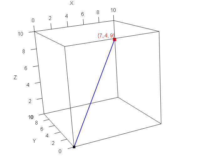
Here the blue line is a vector from the origin to the relevant point in space (the red mark). Visualizing a document in 5 dimensions is trickier, but the principle is the same. To make everything more explicit we might write it like this, where each column is the token in question.
| cat | mat | on | sat | the |
|---|---|---|---|---|
| 1 | 1 | 1 | 1 | 2 |
Let’s add another document. It is
the parrot sat on the perch
We now have:
| cat | mat | on | parrot | perch | sat | the | |
|---|---|---|---|---|---|---|---|
| Document 1 | 1 | 1 | 1 | 0 | 0 | 1 | 2 |
| Document 2 | 0 | 0 | 1 | 1 | 1 | 1 | 2 |
This added a couple of words to the vocabulary of the corpus, so we see some zeros: the first document doesn’t use parrot or perch; the second doesn’t use cat and mat
This structure, with the words as columns and the rows as documents is called the Document-Term Matrix (DTM), or the Document-Feature Matrix (DFM). Each cell of this matrix contains the frequency of the relevant single word (“unigram counts”) involved.
Finally, for our analysis in this chapter, we will calculate the similarity of a few example documents in order to evaluate the similarity of texts.
9.2.7 Document Similarity
- Euclidean Distance: this is the ordinary “straight line” distance between two points. We met it before when we were using kNN classification. Recall that for two points, \(\mathbf{p}\) and \(\mathbf{q}\) it is
\[ D(\mathbf{p},\mathbf{q}) = \sqrt{ (p_0-q_0)^2 + (p_1-q_1)^2+ \ldots +(p_m - q_m)^2 } \] The key is that we can think of the documents as just instances of \(\mathbf{p}\) and \(\mathbf{q}\). In particular, let just use the documents from the document term matrix above. In that case, we have:
\[\begin{align*} D(\mathbf{p}, \mathbf{q}) &= \sqrt{(1 - 0)^2 + (1 - 0)^2 + (1 - 1)^2 + (0 - 1)^2 + (0 - 1)^2 + (1 - 1)^2 + (2 - 2)^2} \\ &= \sqrt{1^2 + 1^2 + 0^2 + (-1)^2 + (-1)^2 + 0^2 + 0^2} \\ &= \sqrt{1 + 1 + 0 + 1 + 1 + 0 + 0} \\ &= \sqrt{4} \\ &= 2 \end{align*}\]
or
euclidean_distance <- function(p, q) {
  sqrt(sum((p - q)^2))
}

# Example usage:
p <- c(1, 1, 1, 0, 0, 1, 2)
q <- c(0, 0, 1, 1, 1, 1, 2)

euclidean_distance(p, q)
This turns out to be 2. This distance is increases the more different the documents are, in terms of their counts. For example, let’s suppose we have third document that is the same as \(\mathbf{q}\) except we just multiple each element by 3. Then we have:
## [1] 6.63325which is reuclidean_distance(p, q3)`. Suppose though that this third document is just the second one reported three times. In some sense, it isn’t really different in content terms to \(\mathbf{q}\) and we might want to be cautious about over-interpreting that larger distance.
One way to deal with such problems is to use
- Cosine similarity: a metric to calculate the distance between two documents in terms of the cosine of the angle between two vectors projected in a multi-dimensional feature space. This sounds complicated, but the key element is that we find a way to divide out by the length of the documents. Here, that means we take into account how large the token counts are.
More specifically, the cosine similarity between two vectors \(\mathbf{p}\) and \(\mathbf{q}\) is defined as:
\[ \text{cosine similarity}(\mathbf{p}, \mathbf{q}) = \frac{\mathbf{p} \cdot \mathbf{q}}{\|\mathbf{p}\| \, \|\mathbf{q}\|} \]
Where:
- \(\mathbf{p} \cdot \mathbf{q} = \sum_{i=1}^n p_i q_i\) and is known as the “innner product” of \(\mathbf{p}\) and \(\mathbf{q}\).
- \(\|\mathbf{p}\| = \sqrt{\sum_{i=1}^n p_i^2}\) and is known as the “Euclidean norm” of \(\mathbf{p}\)
- \(\|\mathbf{q}\| = \sqrt{\sum_{i=1}^n q_i^2}\) and is known as the “Euclidean norm” of \(\mathbf{q}\)
The larger the similarity, the more similar the documents are. The smaller the similarity, the more different they are. Here’s a simple piece of code for this new measure:
#   cosine similarity
cosine_similarity <- function(p, q) {
  dot_product <- sum(p * q)
  norm_p <- sqrt(sum(p^2))
  norm_q <- sqrt(sum(q^2))
  similarity <- dot_product / (norm_p * norm_q)
  return(similarity)
}

# Calculate and print cosine similarity
cosine_similarity(p, q)
## [1] 0.75Let’s double check the similarity between \(\mathbf{}\) and \(\mathbf{q3}\), our new document:
## [1] 0.75So, because we now normalize by length, this was the same as previously. This will be important in some applications.
9.2.8 TF-IDF
To this point, we have been assuming that all features—all terms—should be an equal footing. That is, we have just counted them, with no special weighting based on, for example, how common or rare they are. A popular alternative to basic “term frequency” is “term frequency-inverse document frequency” (TF-IDF). We will explain the formula, but the intuition is that we find a way to weight up terms that are distinctive to particular documents. And, conversely, we find a way to weight down—diminish the importance of—terms that are common across documents, like the, and, a etc. This is very useful when we want to understand what a document is about relative to other documents.
The formula is:
\[ \text{TF-IDF} = \text{TF} \times \text{IDF} \] Here:
- TF, is term frequency. This is just the number of times a given word appears in a document.
- IDF is inverse document frequency. This is usually
\[ \log\left(\frac{\text{size of corpus}}{\text{number of documents containing that word}}\right) \] If you don’t know how to use logs, that’s fine for now: just think of it as an operation that down-weights extreme values of what it is applied to.
In his 1933 inaugural address, FDR used will 10 times. So TF\(=10\). Across all his four inaugural addresses he used it in every speech. The IDF of will for this corpus is
\[ \log\left(\frac{\text{size of corpus}}{\text{number of documents containing that word}}\right) = \log\left(\frac{4}{4}\right) \] which is 0. If we multiply that by the term frequency, we get zero.
What about the term expect? FDR used expect once in 1933 and then never again. So the TF is 1, and the IDF is
\[ \log\left(\frac{\text{size of corpus}}{\text{number of documents containing that word}}\right) = \log\left(\frac{4}{1}\right) \]
which is 1.38 (if we use natural log)—this is the weight that the term expect gets in this corpus.
Note how the TF-IDF weight is specific to this term in this specific document: it is not the same for every document that uses the same term.
9.3 Working with Quanteda
We will now work through some of the steps we mentioned in the previous document, using the quanteda package in R.
9.3.1 Making a corpus
We will make a couple of documents, just by using vector notation. There are much easier more efficient ways to read in multiple files if we need to, but we’ll cover those later. So:
doc1 <- c("The nonpartisan Congressional Budget Office said Wednesday that the broad Republican bill to cut taxes and slash some federal programs would add $2.4 trillion to the already soaring national debt over the next decade, in an analysis that was all but certain to inflame concerns that President Trump’s domestic agenda would lead to excessive government borrowing.")

doc2 <- "At the same time, Republicans have targeted programs that help low-income Americans for cuts. Under the House-passed version of the legislation, nearly 11 million Americans are expected to lose health coverage, for example. The loss in those benefits would overwhelm the modest savings that Americans on the lower rungs of the income ladder would see from tax cuts.

Even with the cuts to safety-net programs, the legislation would still be costly, with the budget office previously estimating that it would add nearly $3 trillion to the debt over the next decade, including additional borrowing costs."
We will put these in corpus:
## Corpus consisting of 2 documents.
## text1 :
## "The nonpartisan Congressional Budget Office said Wednesday t..."
##
## text2 :
## "At the same time, Republicans have targeted programs that he..."
This just holds our documents, as text1 and text2.
9.3.2 Preprocessing
Let’s do some preprocessing. The key function will be tokens and various derivatives thereof. In particular, take a look at
?tokensand all the possible options. For now, we will lower-case everything using tolower and remove punctuation and numbers:
# lowercase
tokens_lower <- tolower(our_corpus)

# remove punctuation and numbers
tokens_cleaned <- tokens(tokens_lower, remove_punct = TRUE, remove_numbers = TRUE)
We can take a look at the first document, just to get a sense of how it has been changed:
## Tokens consisting of 1 document.
## text1 :
##  [1] "the"           "nonpartisan"
##  [3] "congressional" "budget"
##  [5] "office"        "said"
##  [7] "wednesday"     "that"
##  [9] "the"           "broad"
## [11] "republican"    "bill"
## [ ... and 44 more ]
So far so good, but we probably want to get rid of the English (en) stop words too:
Finally let’s stem the corpus and move everything into a document feature matrix using dfm:
# stem it
stemmed_corpus  <-tokens_wordstem(tokens_no_stops, language = "english")

# make it into a dfm:
corpus_dfm <- dfm(stemmed_corpus)
We can take a look at the document feature matrix:
## Document-feature matrix of: 2 documents, 68 features (40.44% sparse) and 0 docvars.
##        features
## docs    nonpartisan congression budget offic
##   text1           1           1      1     1
##   text2           0           0      1     1
##        features
## docs    said wednesday broad republican bill
##   text1    1         1     1          1    1
##   text2    0         0     0          1    0
##        features
## docs    cut
##   text1   1
##   text2   3
## [ reached max_nfeat ... 58 more features ]
As you can see, we are now down to just 68 features (words), and there are lots of zeros (which makes sense, because not all documents use the same words). Still, we have done a good job and reducing the complexity of the documents relative to when we started. At that point, there were (at least, depending on how you count) this many unique features:
## [1] 1029.3.3 Key Words in Context
Before we get too heavily into more abstract processing and distances, it can be good to remind ourselves exactly how people are using tokens. Here we can turn to “key words in context”, which does exactly what it suggests: it shows where words are being used relative to other words, such that we can make a little more sense of their meaning in our documents. For example, we might want to know how people use the term `budget’ in a particular corpus.
In quanteda, we can use the kwic function. Here we apply it to the tokenized corpus:
## Keyword-in-context with 2 matches.
##   [text1, 4] nonpartisan congressional |
##  [text2, 73]                  with the |
##
##  budget | office said
##  budget | office previously
We set the window to “2” here, meaning we get two words either side. But that’s enough to note that the documents are talking about the budget in terms of the Budget office.
9.3.4 Distances
We can calculate the distances and similarities “manually” using our functions, or we can use the built-in ones from the add-on quanteda.textstats package. Let’s do that:
And now:
# Compute Euclidean distance
euclidean_dist <- textstat_dist(corpus_dfm, method = "euclidean")

# Compute Cosine similarity
cosine_sim <- textstat_simil(corpus_dfm, method = "cosine")
The results here are stored as symmetric matrices: the distance between document 1 and document 2 is the same as the distance between 2 and 1. And the distance between a document and itself is 0; the similarity between a document and itself is 1. Thus:
## textstat_dist object; method = "euclidean"
##       text1 text2
## text1     0  8.77
## text2 8.77 0## textstat_simil object; method = "cosine"
## text1 text2
## text1 1.000 0.314
## text2 0.314 1.0009.3.5 TF-IDF
Here’s a specific example of TF-IDF using quanteda’s built-in data. Let’s load that up:
Then, let’s subset to FDR’s inaugural speeches.
# Subset FDR's inaugural addresses (1933, 1937, 1941, 1945)
fdr_corpus <- corpus_subset(data_corpus_inaugural,
                            President == "Roosevelt" & Year %in% c(1933, 1937, 1941, 1945))

# Tokenize and create a document-feature matrix (dfm)
dfm_raw <- dfm(tokens_tolower(tokens(fdr_corpus, remove_punct = TRUE)))
In his 1933 inaugural address, FDR used will 10 times. We can see this via
## Document-feature matrix of: 4 documents, 1 feature (0.00% sparse) and 4 docvars.
##                 features
## docs             will
##   1933-Roosevelt   10
##   1937-Roosevelt   15
##   1941-Roosevelt    4
##   1945-Roosevelt    7
So TF\(=10\). Across all his four inaugural addresses he used it in every speech. The IDF of will for this corpus is
\[ \log\left(\frac{\text{size of corpus}}{\text{number of documents containing that word}}\right) = \log\left(\frac{4}{4}\right) \] which is 0. If we multiply that by the term frequency, we get zero.
What about the term expect? FDR used expect once in 1933 and then never again:
## Document-feature matrix of: 4 documents, 1 feature (75.00% sparse) and 4 docvars.
##                 features
## docs             expect
##   1933-Roosevelt      1
##   1937-Roosevelt      0
##   1941-Roosevelt      0
##   1945-Roosevelt      0
So the TF is 1, and the IDF is
\[ \log\left(\frac{\text{size of corpus}}{\text{number of documents containing that word}}\right) = \log\left(\frac{4}{1}\right) \]
which is 1.38 (if we use natural log)—this is the weight that the term expect gets in this corpus.
We can double-check this using quanteda’s functions:
# Apply tf-idf weighting
dfm_tfidf <- dfm_tfidf(dfm_raw, base= exp(1))

# then, compare:
dfm_tfidf[,"will"]
## Document-feature matrix of: 4 documents, 1 feature (0.00% sparse) and 4 docvars.
## features
## docs will
## 1933-Roosevelt 0
## 1937-Roosevelt 0
## 1941-Roosevelt 0
## 1945-Roosevelt 0## Document-feature matrix of: 4 documents, 1 feature (75.00% sparse) and 4 docvars.
## features
## docs expect
## 1933-Roosevelt 1.386294
## 1937-Roosevelt 0
## 1941-Roosevelt 0
## 1945-Roosevelt 0Again, notice how the TF-IDF weight is specific to this term in this specific document: it is not the same for every document that uses the same term.
9.4 Naive Bayes
Suppose we want to allocate a given email to one of two locations in our email program: it is spam or `ham’ (our term for non-spam). The only information we have available to do this is the words the emails contain, and their frequency. That is, we will assume for now we don’t have meta-data like the sender address or the time it arrived in our inbox.
The particular classifier we will use here is called Naive Bayes. It is naive insofar as it will make some very bold assumptions about the data. These will almost always be wrong but are nonetheless very helpful. It is called Bayes insofar as it uses Bayes’s Law. It goes by other names too, like simple Bayes or Independence Bayes. As we will see, this family of classifier is very fast and simple, and often very accurate. Unsurprisingly, it is very popular.
9.4.1 Set-Up
We’re interested in the probability that an email is in a given category (spam v ham), given its features—i.e. frequency of terms. The conditional probability of a term \(t_k\) occurring in a document, given that document is of class \(c\), is \(=\Pr(t_k|c)\).
For example, it might be that \(\Pr(\texttt{beneficiary}|\texttt{spam})=0.9\). This means: the probability that an email contains the words beneficiary given it is spam is 0.9—so very high. This is telling us implicitly that a lot of spam emails use this term. Perhaps \(\Pr(\texttt{beneficiary}|\texttt{ham})=0.04\). This is telling us implicitly that non-spam emails do not use this term very often: you would expect to find it rarely among all the ham emails. As usual, we are making the bag of words assumption and we’re not taking word order or location into consideration.
We can write the probability that a given email \(d\) contains all the terms, if it’s from a class \(c\), as
\[
\Pr(d|c)=\prod^{K}_{k=1}\Pr(t_k|c)
\]
This formula looks intimidating but is not. A document \(d\) is just an email. And for us the thing we call an “email” is just the collection of words it contains. That is \(\text{term}_1\) which might be dear, \(\text{term}_2\) which might be today, \(\text{term}_3\) which might be best and so on.
The letter \(c\) just denotes whether we are talking about spam or ham. Let’s suppose for now we are talking about the spam category.
The product sign \(\prod\) is telling us that if you want to know how likely you are to see this particular collection of words in an email given you are looking only at spam emails, it is just the probability of seeing the first term given you are in spam, times by the probability of the second term given you are looking only at spam, times by the probability of the third term given you are only looking at spam and so on.
This may not be obvious, but we are multiplying everything together in this way because we are assuming the terms occur independently of each other. That is, seeing dear doesn’t make sir more likely or seeing dollars doesn’t make cents more likely and so on. This is obviously false, but we will see how it works out for us.
9.4.2 Using Bayes Theorem
In any case though, the thing we’ve calculated is not the thing we actually want. We have calculated the \(\Pr(d|c)\). This is the probability of seeing this collection of term in an email, given the email is spam. But we don’t know if the email is spam—we are trying whether it is or not so we can filter it out or not.
So what we actually want is \(\Pr(c|d)\): the probability that this document is from spam given the words it contains. Fortunately we have a machine that can take us from \(\Pr(d|c)\) to \(\Pr(c|d)\) and that machine is called *Bayes Theorem** (or Bayes Rule, or Bayes Law).
Generically for any conditional probability we know that
\[ \Pr(A|B) = \frac{\Pr(A,B)}{\Pr(B)} \] In words: the probability of event \(A\) occuring given event \(B\) has occurred is the probability of \(A\) and \(B\) occurring, divided by the probability of (just) event \(B\) occurring. A much more useful way to express this, however is:
\[ \Pr(A|B) = \frac{\Pr(A)\Pr(B|A)}{\Pr(B)} \]
Where
- \(\Pr(A)\) is the probability of \(A\) occurring, called our prior on \(A\)
- \(\Pr(B|A)\) is the probability of \(B\) occurring given \(A\) occurred. This is sometimes called the likelihood of the data.
Notice that we now have \(\Pr(A|B)\) expressed in terms of \(\Pr(B|A)\). But that means we can express \(\Pr(c|d)\) in terms of \(\Pr(d|c)\) which is what we wanted. So:
\[ \Pr(c|d)=\frac{\Pr(c)\Pr(d|c)}{\Pr(d)} \]
But we can actually simplify even further. Notice that the denominator, \(\Pr(d)\) doesn’t affect whether a given value of \(c\) is more or less plausible. The denominator doesn’t involve \(c\) at all. Because of this, we can drop the denominator altogether, and write
\[ \Pr(c|d) \propto \Pr(c)\Pr(d|c) \] The \(\propto\) symbol means “proportional to”. It’s telling us that when the quantity on the right hand side increases, the thing we care about—\(\Pr(c|d\)—is larger. When the quantity on the right hand side decreases, the thing we care about—\(\Pr(c|d\)—is also lower. It’s not telling us exactly how much higher or lower it is, but we’ll see we don’t need that.
Just substituting in the terms we had earlier, we now see that:
\[ \Pr(c|d)\propto\underbrace{\Pr(c)}_{\mathrm{prior}}\;\;\underbrace{\prod^{K}_{k=1}\Pr(t_k|c)}_{\mathrm{likelihood}} \]
9.4.2.1 Aside: Derivation of Bayes Rule
If you’re interested, here is how Bayes Rule is derived. We said that
\[ \Pr(A|B) = \frac{\Pr(A,B)}{\Pr(B)} \]
Let’s write the same expression but in terms of \(B|A\). Then:
\[ \Pr(B|A) = \frac{\Pr(B,A)}{\Pr(A)} \]
But the probability of \(A\) and \(B\) occuring is the same as the probability of \(B\) and \(A\) occurring. That is, \(\Pr(A,B)=\Pr(B,A)\). From the second equation, we also know that
\[ \Pr(B,A)={\Pr(A)}\times \Pr(B|A) \] But if this quantity is also equal to \(\Pr(A,B)\), it must be that
\[ \Pr(A|B) = \frac{\Pr(A)\Pr(B|A)}{\Pr(B)} \]
9.5 Using Naive Bayes
We want to classify new data (emails), based on patterns we observe in our training set (which we will classify by hand). For example, we might look at 10,000 emails to this point in time, and classify them as being in spam or ham. That is, \(c\in\{\texttt{spam},\texttt{ham}\}\). We use that information, and the terms associated with the two classes, to categorize tomorrow’s email.
In particular, we typically want to assign the document—the email— to a single best class. We have a special name for this ‘best’ class. It is the maximum a posteriori class, or \(c_{map}\). It is whatever class leads to the highest \(\Pr(c|d)\) for this particular email in front of us. Intuitively, it is the answer to the question “of the two classes, which seems most plausible as a place to assign this email?”
Where do we get the various quantities we need? Well, we want
\[ \Pr(c|d)\propto\underbrace{\Pr(c)}_{\mathrm{prior}}\;\;\underbrace{\prod^{K}_{k=1}\Pr(t_k|c)}_{\mathrm{likelihood}} \]
- the likelihood, \(\prod^{K}_{k=1}\Pr(t_k|c)\) comes from multiplying all the probabilities we discussed above, together. We get a given probability, like \(\Pr(\texttt{dollar}|\texttt{spam})\) by asking how often the word occurs in the spam emails (in the training set), divided out the total number of words we saw in the emails.
- the prior, \(\Pr(c)\) we can get from anywhere, but the logical place is just proportion of documents in our training data that are
spamorhamrespectively. This will sum to one.
9.5.1 An example
Let’s work through an example. In our training set, we have 5 emails. We list there words (clearly we have stemmed or stopped out a bunch of other terms), and then whether we human-coded them as spam or ham.
| words | classification | ||
|---|---|---|---|
| training | 1 | money inherit prince | spam |
| 2 | prince inherit amount | spam | |
| 3 | inherit plan money | ham | |
| 4 | cost amount amazon | ham | |
| 5 | prince william news | ham | |
| test | 6 | prince prince money | ? |
Now a new email comes in, and we want to know which category it belongs to. The email consists of three words: prince, prince, money.
Our prior on it being ham is just how common ham was in our training set. So, 3 out of 5, or \(\frac{3}{5}\). We calculate the likelihood as
\[ \Pr(\texttt{prince}|\texttt{ham}) \times \Pr(\texttt{prince}|\texttt{ham}) \times \Pr(\texttt{money}|\texttt{ham}) \]
We get those quantities directly from the training set. Among the ham emails, the probability of seeing prince was \(\frac{1}{9}\). This is literally the fraction of all terms in ham that were prince. The probability of seeing money was \(\frac{1}{9}\) for similar reasons. So, the likelihood is
\[ \frac{1}{9}\times \frac{1}{9}\times \frac{1}{9} = \frac{1}{729} \] Now, we can combine that with the prior to obtain \(\Pr(\texttt{ham}|d)\), or rather, something proportional to it:
\[ \Pr(\texttt{ham}|d) \propto \frac{3}{5} \times \frac{1}{729} = 0.00082. \]
Using the same logic for \(\Pr(\texttt{spam}|d)\), we get:
\[ \Pr(\texttt{spam}|d) \propto \frac{2}{5} \times \frac{2}{6} \times \frac{2}{6} \times \frac{1}{6} . \]
This is
\[ \Pr(\texttt{spam}|d) \propto 0.0074 \]
Clearly, the \(\Pr(\texttt{spam}|d)\) is much larger than \(\Pr(\texttt{ham}|d)\), so our prediction given the data is that the email is spam. Another way to put this is that spam is our maximum a posteriori class or \(c_{\text{map}}\). Notice that we didn’t need to calculate the exact probability of spam or ham: we just had to work out which probability was larger.
9.5.2 Using R for naive Bayes
We can perform the same analysis much more quickly using quanteda. First, we create the relevant corpus:
require(quanteda)
require(quanteda.textmodels)
email1 <- c("money inherit prince")
email2 <- c("prince inherit amount")
email3 <- c("inherit plan money")
email4 <- c("cost amount amazon")
email5 <- c("prince william news")
email6 <- c("prince prince money")
the_corpus <- corpus(c(email1, email2, email3, email4, email5, email6))
docvars(the_corpus, "category") <- c("spam", "spam", "ham", "ham", "ham", NA)

# make into a dfm
dfm_corp <- dfm(tokens(the_corpus))

# Split into training and test sets
dfm_train <- dfm_corp[1:5, ]
dfm_test  <- dfm_corp[6, ]

# Fit Naive Bayes model
nb_model <- textmodel_nb(dfm_train, docvars(the_corpus, "category")[1:5])

# Predict category of email6
prediction <- predict(nb_model, newdata = dfm_test)

# View result
print(prediction)
## text6
## spam
## Levels: ham spamWe can double-check our working above:
##
## docs          ham      spam
##   text6 0.2045827 0.7954173