7 Logistic Regression
7.1 Background
We were previously working with linear regression for continuous outcomes, like house prices. But it’s not hard to think of binary outcomes that occur in social science, that is, cases where \(Y\)—the variable we are trying to predict or explain—takes one of two values.
For example:
- voters turn out to vote, or they don’t
- a bill is passed, or it isn’t
- a war occurs between two countries, or it doesn’t
In all these cases we can code \(y_i=1\), and \(y_i=0\), respectively. Sometimes \(y_i=1\) is referred to as a success, \(y_i=0\) is a failure, even though that doesn’t fit the substantive background of the problem. And, in fact, you can define a success or failure to be whatever you want for your particular problem.
Just as a note for future studies, when \(Y\) is not continuous (or is restricted in some way), we sometimes refer to it as a “limited dependent variable”.
7.1.1 Understanding Probability
Suppose there are 7 Politics majors in POL 346, and 4 Econ majors. As a proportion, we have \(\frac{7}{11}=0.64\) Politics, \(\frac{4}{11}=0.36\) Econ.
Now imagine I draw a person at random from the class, what is the probability they are a Politics major? Well, I get 7 chances in 11, so 0.64. And Econ? 0.36.
We will write \(\Pr(\text{Politics})=0.64\), which in this case is the same as saying \(\Pr(y_i=1)\). The probability of an Economist can be written as \(\Pr(y_i=0)\). Notice that when the possibilities are binary, the probability that \(y_i=1\) is equal to
\(1 - \text{probability that } y_i=0\). Or more concisely: \(\Pr(y_i=1) = 1 - \Pr(y_i=0)\)
7.1.2 Running Example
We want to know why people turnout to vote. So, \(y_i \in \{0,1\}\). This means: “the dependent variable (\(y_i\)) can take the value zero or one for an individual”. In this case, we will say \(y_i=1\) if they go and vote, and \(y_i=0\) if they do not.
We think the decision to turnout, we think it probably depends (positively) on income, that is, we think as people become richer, they are more likely to vote. But we also suspect the effect of income might not be “linear.” For example, we don’t think that adding $1000 to the income of someone earning $200,000 has the same effect as adding $1000 to the income of someone earning $2500. Specifically, we think a rich person is already pretty likely to vote, such that adding another $1000 won’t make much difference.
What should we do about this sort of problem? Let’s start by looking at some data (admittedly simulated). We will plot turnout (0/1) against income in thousands of dollars.
voting_data <- read.csv("data/voting_data.csv")

# color vector
cols <- voting_data$turnout
cols[cols=="1"] <- "darkgreen"
cols[cols=="0"] <- "red"


plot(voting_data$income, voting_data$turnout, bg=cols, col="black",
     pch=21, cex = 2,
     xlab="income ($k)", ylab="voted")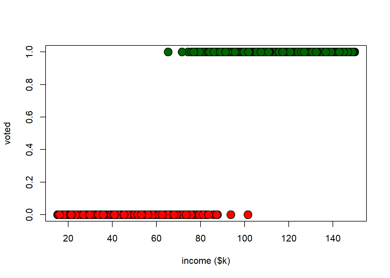
It should be obvious from this plot, but higher income is positively associated with turning out to vote. We can look at correlations and histograms to confirm:
## [1] 0.8582543par(mfrow=c(2,1))
hist(voting_data$income[voting_data$turnout==0], col="red", xlab="", main="non-voters")
hist(voting_data$income[voting_data$turnout==1], col="darkgreen",
xlab="", main="voters")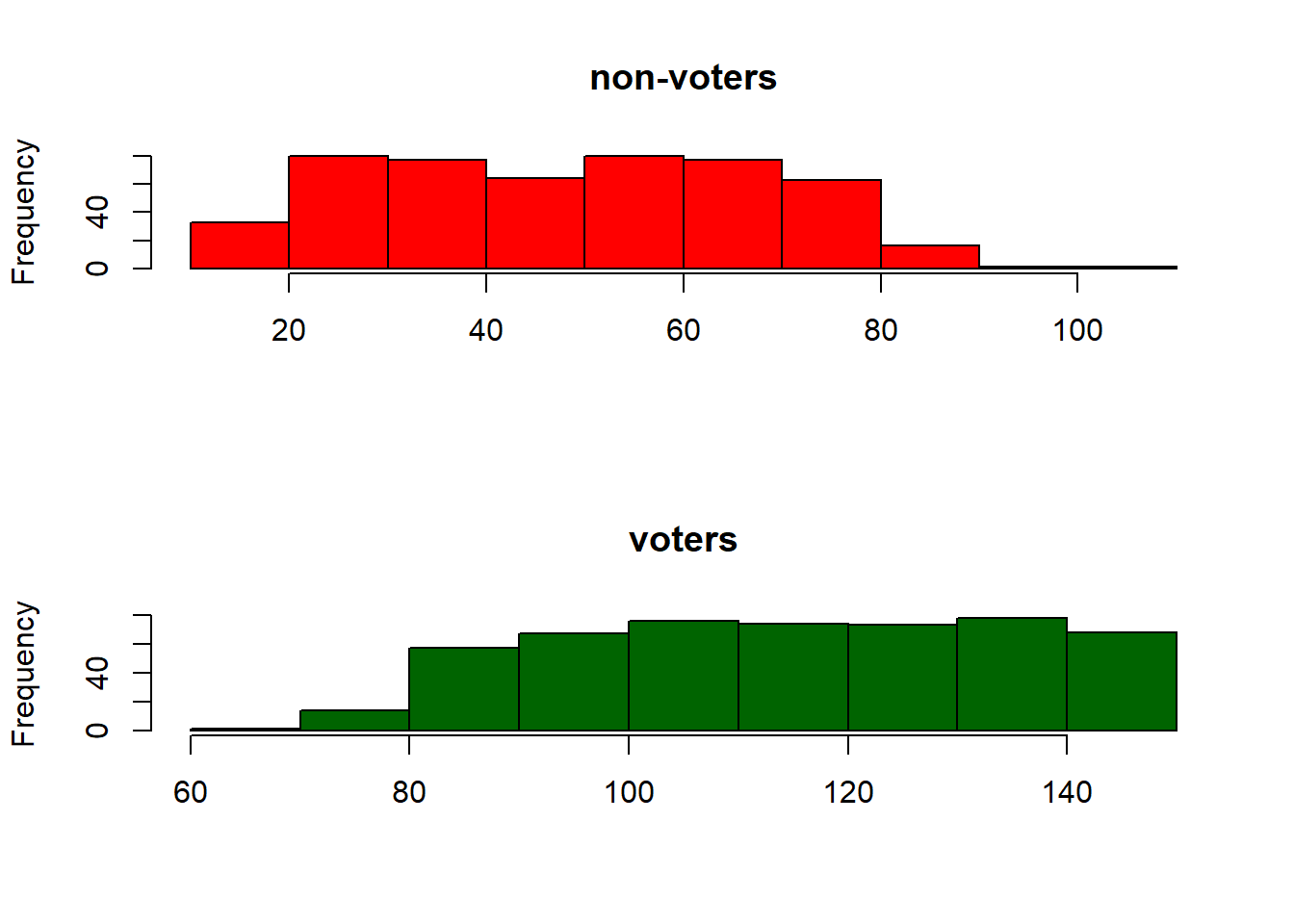
7.1.3 Using the Linear Model
Even though the dependent variable is binary valued, there’s no technical issue with using the linear model. The relevant coefficient table is
##
## Call:
## lm(formula = turnout ~ income, data = voting_data)
##
## Residuals:
##      Min       1Q   Median       3Q      Max
## -0.72188 -0.19393  0.00699  0.18032  0.67801
##
## Coefficients:
##               Estimate Std. Error t value
## (Intercept) -0.4004801  0.0190181  -21.06
## income       0.0110612  0.0002094   52.83
##             Pr(>|t|)
## (Intercept)   <2e-16 ***
## income        <2e-16 ***
## ---
## Signif. codes:
## 0 '***' 0.001 '**' 0.01 '*' 0.05 '.' 0.1 ' ' 1
##
## Residual standard error: 0.2568 on 998 degrees of freedom
## Multiple R-squared:  0.7366, Adjusted R-squared:  0.7363
## F-statistic:  2791 on 1 and 998 DF,  p-value: < 2.2e-16
This is telling us that for every $1000 extra income, \(Y\) increases by 0.0110612 units. What are the units of turnout? Well, one possibility is to think of \(Y\) as a probability. For each \(x\)-value, the OLS line yields a predicted probability that a person with that \(x\)-value will vote. That line will look something like this:
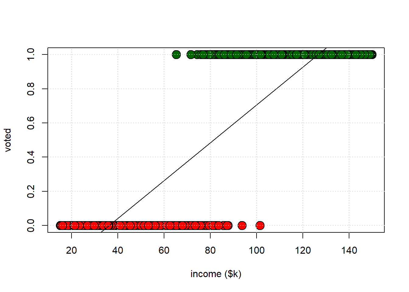
This approach is called the linear probability model (LPM) for obvious reasons. It is very popular in econometrics, but less popular in statistics. What are some reasons we might not want to use it? Some criticisms of the LPM include:
- predicted probabilities can be estimated as being less than zero and more than one, which doesn’t make sense
- the marginal effects can be misleading: basically, the LPM insists that the effect of \(X\) on \(Y\) is always the same (constant) value of \(\hat{\beta}\), but we could imagine situations where it might vary as the value of \(X\) varies.
- it can be hard to compare fit across models, especially if you want to penalize for numbers of variables
- some technical reasons to do with having to assume “homoskedastic” errors for LPM, when those may not apply.
How much one should care about any of these things is hotly debated, but we will take a look at a couple of them and the way that this might motivate logistic regression
7.2 Logistic Regression
7.2.1 What’s “wrong” with the LPM?
Let’s return to our LPM plot, except this time with a larger \(y\) axis. Take a look at the orange and purple points. The purple point is our prediction for someone earning \(\$145k\) a year. The orange point is our prediction for someone earning \(\$18k\) a year. Read across to the \(y\)-axis to see what their predicted probability of voting is.
##
## Call:
## lm(formula = turnout ~ income, data = voting_data)
##
## Residuals:
##      Min       1Q   Median       3Q      Max
## -0.72188 -0.19393  0.00699  0.18032  0.67801
##
## Coefficients:
##               Estimate Std. Error t value
## (Intercept) -0.4004801  0.0190181  -21.06
## income       0.0110612  0.0002094   52.83
##             Pr(>|t|)
## (Intercept)   <2e-16 ***
## income        <2e-16 ***
## ---
## Signif. codes:
## 0 '***' 0.001 '**' 0.01 '*' 0.05 '.' 0.1 ' ' 1
##
## Residual standard error: 0.2568 on 998 degrees of freedom
## Multiple R-squared:  0.7366, Adjusted R-squared:  0.7363
## F-statistic:  2791 on 1 and 998 DF,  p-value: < 2.2e-16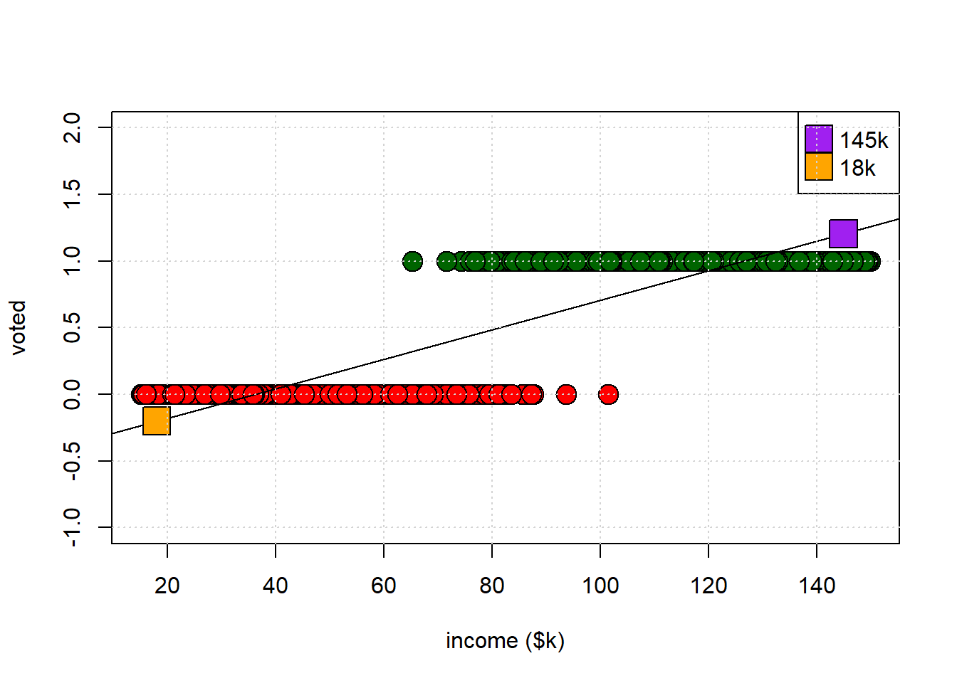
For the low earner, the implied probability is -0.2; for the high earner, it is 1.2. But we cannot have probabilities lower than zero or higher than one, so this seems undesirable. What can we do about this?
7.2.2 Odds and Odds Ratios
Let’s think in a bit more detail about probabilities. If we divide the probability of something happening by the probability of it not happening, we have the odds of that event. So the odds of drawing a Politics major from the class is:
\[ \frac{\Pr(y_i=\text{Politics})}{\Pr(y_i=\text{Econ})} = \frac{\Pr(y_i=\text{Politics})}{1-\Pr(y_i=\text{Econ})} \]
That is:
\[
\frac{0.64}{0.36} = \textbf{1.78}
\]
Thus, “drawing a Politics major is 1.78 times as likely as drawing an Econ major” (which makes sense, because there are almost twice as many Politics majors).
What is the odds of voting for those with salaries between $50k and $90K? We can work it out like this for these earners:
earners <- voting_data[which(voting_data$income<90 & voting_data$income>50),]
how_many_earners <- nrow(earners)
pr_voting <-  sum(earners$turnout == 1)/how_many_earners
pr_not_voting <- sum(earners$turnout == 0)/how_many_earners
odds <- pr_voting/pr_not_voting
print(odds)
## [1] 0.3050847\[ \frac{\Pr(y_i=1 \mid 50 < x_i < 90)}{\Pr(y_i=0 \mid 50 < x_i < 90)} = \frac{72/308}{236/308} \] Because 72 of the 308 in that income band voted, and 236 did not. So, the odds of voting (for this group) is 0.305. They are about a third as likely to vote as not vote.
Alternatively, what are the odds of not voting?
\[
\frac{236/308}{72/308} = 3.277
\]
So this group is a little over 3 times more likely not to vote as to vote. This might be obvious, but note we are dealing with ratios now, so the odds of voting are not equal to \(1 - \text{(odds of not voting)}\). This is just not how odds are defined.
Suppose we also calculate odds of voting for those earning more than $90K:
\[
\frac{436/438}{2/438} = 218
\]
So this group is two hundred times as likely to vote as not vote: essentially everyone votes in this group.
7.2.3 Odds Ratio
We can compare the odds for the two groups. Let’s divide the odds of voting for the high income folks by the odds of voting in the low income group:
\[ \frac{218}{3.277} = 66.5 \]
This is called the odds ratio. Here it tells us that the odds of voting in the richer group are about 66 times greater than the odds in the poorer group. Note that this doesn’t mean the richer group has a probability of voting that’s 66 times larger. It means that their odds are 66 times higher. The jury is out on whether this is helpful to report (!)
7.2.4 What we want: Logistic Regression
One thing we might want to know is how the probability of voting changes systematically as we alter variables on the right-hand side—like income. It would be great if we could just put our explanatory variables (our $Xs) with coefficients for their effects \(\beta\)s on that right hand side, like we do in the usual regression context. As we have seen though, we can’t do it directly with \(y_i \in \{0,1\}\): this gives the LPM, and we said we might not want that set up.
So we need to put something else on the left-hand side (the place we would usually put \(Y\) in a linear regression). The binary outcome, voting or not voting, is still the dependent variable. But we need to find a transformation—a mathematical operation—of the dependent variable that allows us to do our regression in the way we want.
We use the log of the odds and we call it the logit of the probability. We can write the logit as:
\[
\text{logit}(\Pr(y_i = 1)) \quad \text{or}
\quad \log \left( \frac{\Pr(y_i=1)}{1 - \Pr(y_i=1)} \right)
\quad \text{or} \quad\text{logit}(p)
\]
where \(p\) stands in for \(\Pr(y_i = 1)\). We will make this \(\text{logit}(p)\) a linear function of our \(X\)s. So we’ll end up with something like:
\[ \text{logit}(p) = \beta_0 + \beta_1 x_1 + \ldots + \beta_n x_n \] Fitting this model to data, such that we estimate all the \(\beta\)s is called logistic regression.
7.2.4.1 A Note on Logs
The logistic regression uses logs. A log or logarithm is a function that takes a number and returns an exponent to which the base must be raised to get that number.
For example, suppose we have the number 100. Suppose our base is 10. What number do we need to raise 10 to, to get 100? Well, 100 is \(10^{\color{blue}{2}}\), so the answer is 2.
## [1] 100Using base 10 is called the common log. Its antilogarithm requires you take 10 to that number: if you give me 2, I can “get back” to the original number by computing \(10^2 = 100\). In R you can take the log of anything you want (well, so long as the number is not less than or equal to zero) to any base you want:
## [1] 6.643856It turns out that a more popular base in statistics is \(e\) (“Euler’s number”). Here, \(e \approx 2.7\). If we use that base, we are taking the natural log. It’s so popular that most statistical packages use it by default when you call log().
## [1] 6.643856## [1] 4.60517## [1] 4.60517Its antilogarithm is computed by taking \(e\) to that number. So for example
- The antilog of 3 is \(e^3 = 20.09\)
- The antilog of -1.5 is \(e^{-1.5} = 0.223\)
## [1] 100Note: When we take \(e\) to a number \(n\) (\(e^n\)), the absolute result is always greater than zero, though it can be less than 1 if the exponent is negative.
7.3 Working with Logit
Remember the main logistic regression equation: \[ \text{logit}(p) = \beta_0 + \beta_1 x_1 + \ldots + \beta_n x_n. \]
It may not be obvious, but this set up forces the resulting probabilities to always be between zero and one. That’s what we want. The way we estimate the parameters of this model is not the same as with the linear model. And we won’t interpret the results the same way, either.
7.3.1 Estimating a logistic regression
In R, we use the glm() function to estimate a logistic regression (sometimes called a “logit”). The function glm stands for GLM or generalized linear model. A logistic regression is one example of a GLM. In fact, the linear model we have been using up to now is also a special case of a GLM. The way we define GLMs is technical and specific, but one important part is the idea of a “linear predictor”—this means you will find that \(Y\) (your outcome) somehow depends on \(\beta_0 + \beta_1 x_1 + \ldots + \beta_n x_n\) like in the linear regression.
Because there are lots of GLMs, you need to give R specific instructions as to which you want it to fit. Here is the syntax for the logistic regression of turnout on income and renting (i.e. whether you are a renter or someone who owns your property):
The family argument tells R you want a logistic regression, specifically.
7.3.2 Interpreting a Logistic Regression
As with lm we can ask for the regression table:
voting_data <- read.csv("data/voting_data.csv")
logit_model <-glm(formula = turnout ~ income + renter, family = binomial(link = "logit"),
    data = voting_data)
summary(logit_model)
##
## Call:
## glm(formula = turnout ~ income + renter, family = binomial(link = "logit"),
## data = voting_data)
##
## Coefficients:
## Estimate Std. Error z value
## (Intercept) -23.22313 2.64534 -8.779
## income 0.29419 0.03306 8.898
## renter -0.95420 0.41140 -2.319
## Pr(>|z|)
## (Intercept) <2e-16 ***
## income <2e-16 ***
## renter 0.0204 *
## ---
## Signif. codes:
## 0 '***' 0.001 '**' 0.01 '*' 0.05 '.' 0.1 ' ' 1
##
## (Dispersion parameter for binomial family taken to be 1)
##
## Null deviance: 1386.04 on 999 degrees of freedom
## Residual deviance: 158.43 on 997 degrees of freedom
## AIC: 164.43
##
## Number of Fisher Scoring iterations: 97.3.3 Raw Coefficients
Let’s take a closer look at the logit coefficients.
| Estimate | Std. Error | z value | Pr(>|z|) | |
|---|---|---|---|---|
| (Intercept) | -23.2231315 | 2.6453436 | -8.778871 | 0.0000000 |
| income | 0.2941886 | 0.0330614 | 8.898247 | 0.0000000 |
| renter | -0.9542047 | 0.4113996 | -2.319411 | 0.0203728 |
The Intercept tells us the log-odds of voting when the \(X\)s take a zero value.
\(\hat{\beta}\) is “the effect of a one unit change in \(X\) on the log odds”
- So if our \(\hat{\beta}\) on
incomeis 0.29, we say that a one thousand dollar increase in income increases the log-odds of voting by 0.29, holding all other variables constant. - If our \(\hat{\beta}\) on
renteris -0.95, we say that renting (as opposed to buying) decreases the log-odds of voting by -0.95, holding all other variables constant.
We can also take \(e^{\hat{\beta}}\) and:
- if our \(\hat{\beta}\) on
incomeis 0.29, we say that the a one thousand dollar increase in income increases the odds of voting by \(\exp(\hat{\beta})=\exp(0.29)\) which is 1.3364275, holding all other variables constant. - if our \(\hat{\beta}\) on
renteris -0.95, we say that renting (as opposed to buying) decreases the odds of voting by 0.386741, holding all other variables constant.
Neither of these is typically very helpful so we usually just note that:
- if our \(\hat{\beta}\) is positive, this means this variable has a positive effect on the probability of voting (if it increases, we are more likely to vote)
- if our \(\hat{\beta}\) is negative, this means this variable has a negative effect on the probability of voting (if it increases, we are less likely to vote)
A difference between the linear model and the logit is that the latter uses \(Z\) values rather than \(t\) values in the summary table. This is due to the method by which the logit is fit to the data, which is not ordinary least squares. But for our purposes you can interpret the \(p\)-value in statistical significance terms as you would there. So, here, both variables are statistically significant predictors of the outcome.
7.3.3.1 Predicted Probability
We might also want to know the predicted probability of an outcome, contingent on the particular characteristics a given observation has. First, let’s just get the predicted probability for everyone currently in the data. This is obtained by
If we want to look at a specific person already in the data, that’s easy. Here’s observation number 34 and our prediction for them:
##     X turnout   income renter
## 34 34 1 122.3881 0##
## probability of voting == 0.9999972They are a high earner and a house-owner, so we predict they will turnout with a very high probability: 0.99. And, in fact, they did turnout in the real data. But it’s more interesting to think about people not in the data. For example, suppose the person earned $55k a year, and was a renter: what would we predict their probability of voting to be?
new_person <- data.frame(income=55, renter=1)
predict(logit_model, newdata = new_person, type = "response")
## 1
## 0.0003363701That’s pretty unlikely! What about someone who earns $83k but rents? We can work this by hand. First, it turns out that \[ \Pr(y_i=1) = \frac{\text{odds}}{1+\text{odds}} = \frac{\exp(\hat{\beta} X)}{1+\exp(\hat{\beta} X)} \] Well, the log odds for some with this profile is \[ \text{intercept} + \beta_1\times X_1 + \beta_2 \times X_2 \]
which is \[ - 23.22 + 0.294\times83 -0.95\times 1 = 0.232. \] We can then get the odds by taking \(\exp(\hat{\beta}X) = e^{0.232} =1.26\). In which case, the probability is \[ \Pr(y_i=1) = \frac{1.26}{1+1.26} = 0.56 \] In R we do:
new_rich_person <- data.frame(income=83, renter=1)
predict(logit_model, newdata = new_rich_person, type = "response")
## 1
## 0.55979237.3.3.2 Marginal Effects
With the linear model, the marginal effect of a specific \(X\) on \(Y\)—that is, what happens to \(Y\) as we change that \(X\) keeping all other variables constant—was just the \(\hat{\beta}\) on that \(X\). It didn’t matter how many of variables were in the model, or their values.
Things are not so simple with the logistic regression, because the marginal effect of a given \(X\) can change depending on the values the other variables take. For example, the effect of renting (going from renter =0 to renter = 1) on turnout probability can be larger depending on the value of income.
To get a sense of this problem, consider the following code. Here, we move income from $10k a year to $200k, and see what happens to turnout probability. And we do this for people who are renters (in blue) and buyers (in red). In both groups, as income increases, the probability of turnout increases. But the effect is not the same for every level of income.
increasing_income_renter <- data.frame(income=seq(10,200), renter=1)
increasing_income_buyer <- data.frame(income=seq(10,200), renter=0)

renters <- predict(logit_model, newdata = increasing_income_renter, type = "response")
buyers <- predict(logit_model, newdata = increasing_income_buyer, type = "response")

plot(seq(10,200), renters, xlab="income", col="lightblue", type="b",
     pch=16, xlim=c(50,100), ylab="Pr(turnout)")
points(seq(10,200), buyers, col="red", type="b", pch=16)
grid()
legend("topleft", pch=c(16, 16), col=c("lightblue", "red"), legend=c("renters", "buyers"))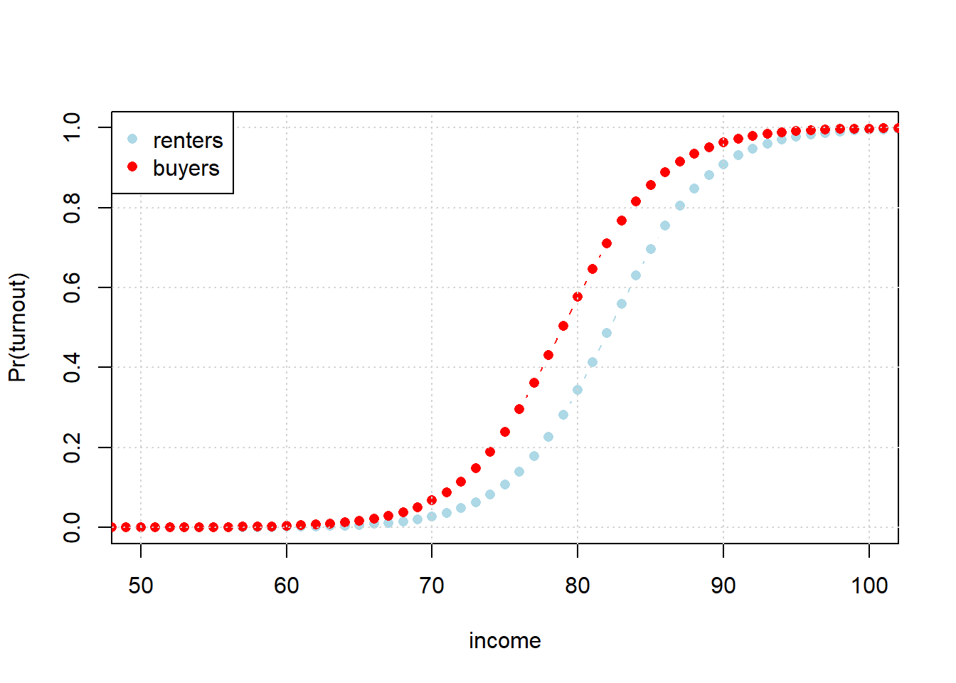
For example, look at the turnout probability when income is $60k: it doesn’t make much difference whether one is a renter or buyer. There’s no gap between the groups, implying renting v buying has no effect. What about at $80k? Here the gap is quite large, with buyers almost twice as likely to vote. But this just makes our point: the effect of renting differs depending on what income group we are talking about. So the effect is not constant. Note, as an aside, how—unlike the LPM—the probability is not linear in the covariate (here income) for either case: the probability curves smoothly (and is always between 0 and 1)
Consequently, we might like a systematic way to summarize the effects of the variables across these sorts of differences. There are lots of different options here, but we’ll look at the most popular option. First, we need the margins package.
We will calculate Average Marginal Effects (AME)—this asks “On average, how does a one-unit change in \(x\) affect the probability of turning out in the data?”
For a given person in the dataset, we first calculate the effect of changing \(x\) (say, income) by one unit, and see what happens to their probabilty of voting. Then we do the same for every other person in the data set, and at the end take the average of all these individual effects.
For our data set, this is
##  factor     AME     SE       z      p   lower
##  income  0.0071 0.0001 66.9272 0.0000  0.0069
##  renter -0.0229 0.0096 -2.3977 0.0165 -0.0417
##    upper
##   0.0073
##  -0.0042
This says that, for income, a one unit ($1000) increase in income increases the probability of voting by 0.0071, on average. However, switching from buying (renter=0) to renting (renter=1) reduces the probablity of voting by 0.0229, on average. This doesn’t mean it’s 0.0071 (or 0.0229) everywhere for everyone, just that on average that is the value.
7.4 More on Logit
7.4.1 Classifying with Logit
As we saw, logistic regression is potentially a good choice when the problem is to predict a binary outcome (0 or 1). That also means it is commonly used in situations where we need to classify observations into two types. As an example, let’s go back to our CKD example from earlier in the semester.
First, we load the data, and create a training and test set.
set.seed(2)
ckd <- read.csv("data/ckd.csv", stringsAsFactors = FALSE)

shuffled_ckd <- ckd[sample(nrow(ckd)), ]
training <- shuffled_ckd[1:79, ]
testing <- shuffled_ckd[80:158, ]
Second, we will set up a logistic regression to predict Class in the training set from a couple of variables
train_model <- glm(Class ~ Blood.Pressure + Hemoglobin, data=training, family = binomial(link = "logit") )Then, we need to predict the relevant outcomes for the test set:
Note that the predictions here are probabilities. A logical next step is compare those to the actual binary class memberships of the test set:
plot(testing$Class, test_predict, pch=21, bg="lightblue", col="black",
     xlab="actual CKD status",
     ylab="predicted probability of CKD", axes=FALSE, cex=2)
axis(1, at=c(0,1))
axis(2)
abline(h=0.5, col="red", lty=2)
grid()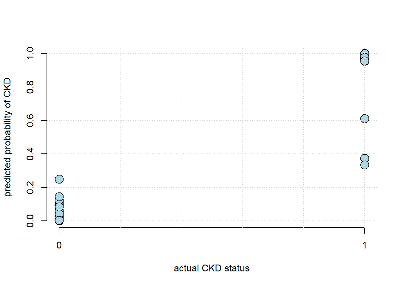
This looks encouraging, insofar as we seem to predict the (true) 1s as having high probability, and the (true) 0s as having low probability. But we would like something more systematic. To do that, we need to convert the predicted probabilities to predicted binary class memberships—that is, zeros or ones.
Typically for a logit, we say that a predicted probability of greater than or equal to one half should be taken as predicting “1”, while anything less than half implies predicting a “0”. Let’s implement that rule:
make_binary_preds <- function(predictions = test_predict){
  predicted_classes <- ifelse(predictions >= 0.5, 1, 0)
  predicted_classes
}
Then, to calculate accuracy, we just need to see how often what we predict for the test set (in binary terms) is what the value of Class actually was in the test set, and then divide by the number of predictions we made. This latter quantity was just the number of observations in our test set.
calc_accuracy <- function(test_set, the_test_predictions){
  bin_preds <-make_binary_preds(the_test_predictions)
  acc <- sum( test_set$Class == bin_preds) / nrow(test_set)
  acc
}

calc_accuracy(testing, test_predict)
## [1] 0.9620253Here, the logit managed \(\sim 96\%\) accuracy.
7.4.2 Probit
We talked about generalized linear models above. They have a linear part on the right-hand side (\(\beta X\)), and then have a non-normal response on the left-hand side, connected via a link function (it provides a bridge from the \(X\)s to the \(Y\)).
We’ve been talking about the logit link function. It relates our linear predictor back to our \(y_i\) via
\[\log\left(\frac{\Pr(y=1)}{1 - \Pr(y=1)}\right)\]
Another option is probit regression. Probit uses a different link function that relies on the normal distribution:
\[\Phi^{-1}(p) = \beta_0 + \beta_1 x_1 + \ldots + \beta_n x_n\]
But generally speaking, probit and logit, for binary \(y\), give extremely similar results (especially in “large” samples). To see this, let’s do a probit version of our logit above, and plot the predicted values relative to the logit.
voting_data <- read.csv("data/voting_data.csv")


logit_model <-glm(formula = turnout ~ income + renter, family = binomial(link = "logit"),
    data = voting_data)
pred_logit <- predict(logit_model, type="response")


probit_model <-glm(formula = turnout ~ income + renter, family = binomial(link = "probit"),
    data = voting_data)
pred_probit<- predict(probit_model, type="response")

par(pty="s")
plot(pred_logit, pred_probit, pch=16,
     xlab="logit", ylab="probit", xlim=c(0,1), ylim=c(0,1))
grid()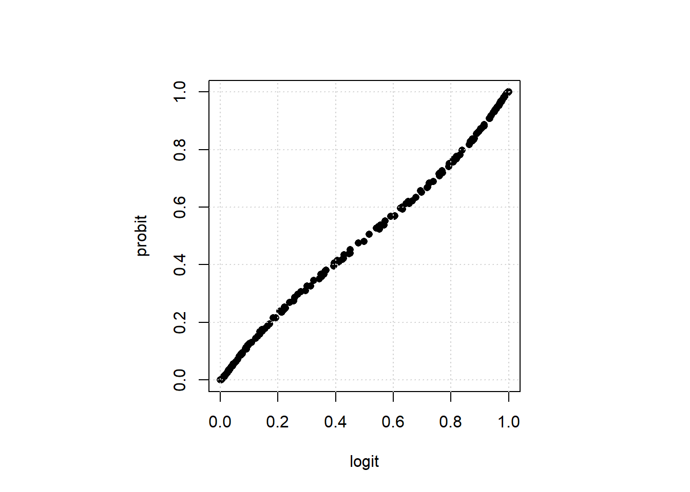
The correlation between there predictions is very high: 0.9997552