8 Panel Data
8.1 Background
Up to now, we’ve mostly been interested in data that allows us to compare units at a given time in terms of their outcomes. For example, in the Snow case, he was interested in households in London in 1854. Had he recorded the data for Soho systematically, it might have looked something like this:
| Household | Drinks_from_pump | Cholera |
|---|---|---|
| 1 Broad Street | 1 | 1 |
| 3 Broad Street | 1 | 1 |
| 5 Broad Street | 0 | 0 |
| 1 Wick Street | 0 | 1 |
| 2 Wick Street | 1 | 1 |
| Lion Brewery, Broad Street | 0 | 0 |
In principle, he could have recorded this data over time, say every month in 1854. In that case, it might look more like this:
| Household | Date | Drinks_from_pump | Cholera |
|---|---|---|---|
| 1 Broad Street | August, 1854 | 1 | 1 |
| 1 Broad Street | September 1854 | 1 | 1 |
| 1 Broad Street | November 1854 | 0 | 0 |
| 3 Broad Street | August, 1854 | 0 | 1 |
| 3 Broad Street | September 1854 | 1 | 1 |
| 3 Broad Street | November 1854 | 0 | 0 |
| 5 Broad Street | August, 1854 | 1 | 1 |
| 5 Broad Street | September 1854 | 1 | 1 |
| 5 Broad Street | November 1854 | 0 | 0 |
| 1 Wick Street | August, 1854 | 0 | 1 |
| 1 Wick Street | September 1854 | 1 | 1 |
| 1 Wick Street | November 1854 | 0 | 0 |
| 2 Wick Street | August, 1854 | 1 | 1 |
| 2 Wick Street | September 1854 | 1 | 1 |
| 2 Wick Street | November 1854 | 0 | 0 |
| Lion Brewery, Broad Street | August, 1854 | 0 | 1 |
| Lion Brewery, Broad Street | September 1854 | 1 | 1 |
| Lion Brewery, Broad Street | November 1854 | 0 | 0 |
8.1.1 Cross-section, time series
Whenever we have a cross-section of individual units observed over a time series, we have a panel. There can be lots of units, and a few time periods; or a few units and lots of time periods or some combination thereof. For instance, we observe:
- the same countries over many years
- the same individuals over many months
- the same households over many weeks
These data may be
- balanced meaning we have all data for all units, for all time periods
- unbalanced meaning we are missing some observations for (at least one) units in some (at least one) time periods. The most common way that panels are unbalanced is because a given unit joins or leaves the panel at a time not in keeping with everyone else. For example, we might be looking at countries over the period 1900–2000 and note that the USSR suddenly joins and then suddenly leaves the data set.
Such data is very common in social science. Examples include the British Household Panel survey and the Panel Survey of Income Dynamics. We will now cover some special methods for dealing with this types of data.
8.1.2 Why use Panel Data?
Data in panels can be more helpful than data in cross-sections or time series alone because
- It allows us to deal with heterogeneity in micro-units: by this we mean difference in people or states or households.
Units in a cross-section—like people in a survey or households in Soho—differ from each other in ways that are hard to control for when we we’re trying to produce causal estimates. This might be because we cannot measure the differences easily (as was the case in DiD). As we will see panel data allows us to account for all these unmeasured (time persistent) confounders in one go. Actually, even if there are no confounders, just being able to account for heterogeneity can improve the quality of our estimates.
- It allows us to deal with potential multicollinearity: multicollinearity arises when two variables are so tightly correlated that we cannot control for one while allowing variation on the other—which is what we need to estimate a causal effect. For example, in historical data, it might be the case that all legislators in say 1900 are men. But then we cannot estimate the effect of being a man on, say, speech patterns or ideology. Indeed, we cannot even describe how they vary with being a man or not.
Because panel data allows us to work with a cross section over time, we may be able to introduce more variation and obtain the estimates we want.
- It generally gives us more information—and thus a more complete picture—than time series or cross section data alone.
For instance, suppose that we are interested in the relationship between race and party ID in the South from 1950. If we have a time series only we can see how many people voted Republican or Democrat in a given year. If we have a cross-section only, we can see who voted GOP or Democrat in a given year. If we have panel data we can see if (the same) people are switching parties as time goes by. That is, we can learn something about “internal” unit behavior changes—not just aggregate patterns—that wouldn’t be possible with the other two margins of data alone.
8.1.3 How to use panel data: different intercepts
Panel data is useful because it allows us to model different intercepts for different units in our data (it also allows for different slopes, but we’ll leave that for now). These are baseline differences across units that we might want to take into account. Here are a couple of examples of how and when intercepts might be different for different units:
Suppose we survey the same individuals 2008, 2012, 2016, 2020 and 2024. The outcome \(Y\) of interest is `thermometer feeling towards Republicans, and it can take values between 0–100 (with 100 being the warmest). Our treatment \(X\) of interest is personal income. We can imagine that individual incomes change over time, and that this affects your feeling towards the GOP. We can also imagine that the relationship between income and feeling has the same slope (positive), but that the individuals’ intercepts differs. The intuition is that for some voter specific reason(s), no matter how rich they get, some people just will not like the Republicans as much as others do (even though they feel better disposed towards them). For example, they were brought up in a union household that was pro-Democrat. We cannot observe or measure that upbringing in our data, so it is in the error term from our perspective. A different constant or intercept for each person captures this type of unchanging experience that affects how warmly someone can possibly feel.
Suppose we study the same sub-Saharan African countries are 1951, 1961, 1971, 1981, 1991, 2001, 2011. Our outcome of interest is GDP per capita. Our treatment of interest is whether country has an “extractive” dictator (\(x=1\)) or not (\(x=0\)). We can imagine that dictator-status changes over time, perhaps due to democratization, and this affects a country’s GDP. And we can also imagine that the relationship between dictator-status and GDP has the same slope (negative), but that the countries’ intercepts differ. The intuition is that for some reason(s), no matter their system of government, some countries just will not get as rich as others, even though they get richer relative to their own baseline standard of living. This might be because they have different natural resource endowments, or culture, or property right regimes. We cannot observe or measure that property rights system in our data, so it is in the error term from our perspective. A different constant or intercept for each country this type of unchanging feature that affects how rich that country can get.
In either case we worry that (especially unobserved) things that are specific to the units (like growing up in a union household, or mineral deposits) might affect both the treatment assignment and the outcome. And we would like to deal with that potential confounding somehow. But even if there is no confounding, we still want to take into account heterogeneity so our model is a better fit for reality. Momentarily we will discuss such methods.
To summarize:
- Panel data by definition contains multiple observations (over time) per unit, this allows us to model unit-specific effects (like different intercepts for each person, or country).
- these different intercepts account for unobserved, time-invariant characteristics; for instance, a voter’s upbringing or a country’s natural resource endowments.
8.1.4 Pooled Regression
One popular way to use panel data and allow for different intercepts is via fixed effects. These methods estimate a separate intercept for each unit, which “takes care of” all unchanging characteristics that might otherwise confound the relationship between \(X\) and \(Y\).
To visualize how this works, consider a panel of 13 people, observed over 5 time periods:
| start: time period 1 | time period 2 | time period 3 | time period 4 | end: time period 5 |
|---|---|---|---|---|

|
|
|
|
|
Let’s look at some of these individuals in income v thermometer space:
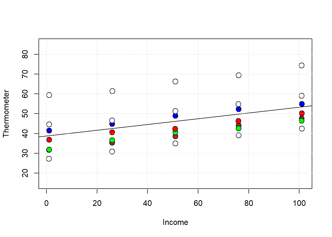
In general, we see that as their careers progressed and their incomes increased (from left to right), they liked the GOP more. The single line on the plot is from the pooled regression of thermometer scaling on income, ignoring any panel structure. That is, it is based on this regression:
##               Estimate Std. Error  t value
## (Intercept) 38.7075948 2.96020508 13.07598
## income       0.1458936 0.04769869  3.05865
##                 Pr(>|t|)
## (Intercept) 1.326132e-14
## income      4.389743e-03
But clearly, the single intercept this pooled regression uses (of around 47) doesn’t reflect the fact the units have different intercepts. But if there have different intercepts (different baseline \(Y\) values), this implies cross-sectional heterogeneity: that is, the voters differ in terms of their other variables (i.e. variables other than \(X\)). If those baseline differences are correlated with \(X\), we might want to control for those differences for the usual reasons: specifically, so that we can make more plausible causal inferences.
8.1.5 Fixed Effects
The idea now is to introduce a different intercept for each person. There’s two main ways to proceed, and we will start with the simplest which is called “fixed effects”—which connotes the (correct) idea that we are dealing with something that is non-random and fixed (for the unit) over time. Other names include the “within estimator” and the “individual dummy model”.
This latter term captures the intuition that it is as if we adding a dummy variable for each person or unit. To recap, a dummy variable is a variable that can only take two values: zero or one. In the Snow case, there will be variables that:
- take the value of “1” if the unit we are dealing with is 1 Broad Street, and zero otherwise—that is, all other units get “0” on this variable.
- take the value of “1” if the unit we are dealing with is 3 Broad Street, and zero otherwise—that is, all other units get “0” on this variable.
- take the value of “1” if the unit we are dealing with is 5 Broad Street, and zero otherwise—that is, all other units get “0” on this variable.
- take the value of “1” if the unit we are dealing with is 1 Wick Street, and zero otherwise—that is, all other units get “0” on this variable.
- …etc etc
…for every household except the last one, which (for various technical reasons) doesn’t need its own dummy if everyone else has one. Ultimately, this adds \(n-1\) variables to the dataset where, recall, \(n\) is the number of units (households or people or countries).
More importantly, adding this dummy wipes out the effect of any other variable that does not change over time in our data: it will just disappear from our regression. This makes sense: if some background factor doesn’t change, it can’t itself have caused any changes in Y. That is, you cannot explain something that’s changing with something that’s constant, so let’s just scrub it. Fixed effects let you do that, and it doesn’t matter whether the background covariate is observed or unobserved.
For example, in our survey above, we think “household as a child” is not changing over time. So whatever effect it has is included in a person’s intercept term, and that’s it. Similarly, “political culture” is not changing (much!) over time. So whatever effect it has on autocracy v democracy should be included in the country’s intercept term, and that’s it.
8.1.5.1 Fitting Fixed Effects
First, let’s do exactly what we suggested above: just add a dummy variable for every unit. In the standard lm setup, this would be equivalent to:
# with base R/lm -- no special packages
fe_base<- lm(thermometer ~ income + factor(respondent), data = gop_panel_data)
summary(fe_base)$coef
## Estimate Std. Error
## (Intercept) 27.469569 0.36241826
## income 0.145873 0.00340183
## factor(respondent)2 4.528194 0.44995106
## factor(respondent)3 4.693291 0.44995106
## factor(respondent)4 8.329712 0.44995106
## factor(respondent)5 13.536973 0.44995106
## factor(respondent)6 16.346578 0.44995106
## factor(respondent)7 31.238796 0.44995105
## t value Pr(>|t|)
## (Intercept) 75.79521 5.355233e-33
## income 42.88073 2.249311e-26
## factor(respondent)2 10.06375 1.238668e-10
## factor(respondent)3 10.43067 5.702166e-11
## factor(respondent)4 18.51248 7.157871e-17
## factor(respondent)5 30.08544 2.652356e-22
## factor(respondent)6 36.32968 1.836325e-24
## factor(respondent)7 69.42710 5.659064e-32the factor(unit) term just reminds lm to treat each different numerical entry in respondent as if it’s a different dummy variable. Actually, what’s really happening here is that we are adding a single variable which takes a different categorical value depending on the observation number, but the effect is the same.
It turns out though that there is a more efficient—in a computational sense—way to fit fixed effects. This involves transforming the data set by subtracting off the mean of each column and then running the relevant linear regression. Packages like fixest can do this for you with a simple call like this:
require(fixest)

# Fixed effects: unit-specific intercepts
fe_model <- feols(thermometer ~ income | respondent, data = gop_panel_data)
summary(fe_model)
## OLS estimation, Dep. Var.: thermometer
## Observations: 35
## Fixed-effects: respondent: 7
## Standard-errors: IID
## Estimate Std. Error t value Pr(>|t|)
## income 0.145873 0.003402 42.8807 < 2.2e-16
##
## income ***
## ---
## Signif. codes: 0 '***' 0.001 '**' 0.01 '*' 0.05 '.' 0.1 ' ' 1
## RMSE: 0.624861 Adj. R2: 0.995917
## Within R2: 0.985529To make the point that fixed effect wipe out time invariant characteristics, let’s compare the pooled model and the fixed effects model with an extra covariate: union_household:
# Fixed effects: unit-specific intercepts
pool2 <- lm(thermometer ~ income + union_household, data=gop_panel_data)
summary(pool2)$coef## Estimate Std. Error
## (Intercept) 42.2977167 2.5890892
## income 0.1458911 0.0392494
## union_household -12.5649731 3.0712821
## t value Pr(>|t|)
## (Intercept) 16.336910 4.396962e-17
## income 3.717026 7.699759e-04
## union_household -4.091117 2.709407e-04Taken at face value, this implies being from a union_household has a negative effect.
For the fixed effects model we would use.
## The variable 'union_household' has been
## removed because of collinearity (see
## $collin.var).Note the warning: this is telling us that, once we use fixed effects, this variable must be dropped. And finally:
## OLS estimation, Dep. Var.: thermometer
## Observations: 35
## Fixed-effects: respondent: 7
## Standard-errors: IID
##        Estimate Std. Error t value  Pr(>|t|)
## income 0.145873   0.003402 42.8807 < 2.2e-16
##
## income ***
## ---
## Signif. codes:  0 '***' 0.001 '**' 0.01 '*' 0.05 '.' 0.1 ' ' 1
## RMSE: 0.624861     Adj. R2: 0.995917
## Within R2: 0.9855298.1.5.2 Interpreting Fixed Effects
Here, using fixed effects made a very small difference to the coefficient on income relative to using a pooled model. But that isn’t always the case. Consider this set of data:
This is (simulated) data on people getting specialty training (like certificates in software support, or a masters in some complex area of law), and how that affects their net worth. The data has been created such that the overall correlation between specialty training and net worth isn’t that large, but for a given individual giving them more specialty training boosts their income a lot especially if they start out relatively poor.
This sort of pattern could emerge because, say, already wealthy people typically select into extra specialty training for prestige reasons; meanwhile, the people for whom it really makes a difference are those who don’t typically recognize its value or cannot take a financial risk on obtaining it.
Now, the true causal relationship between \(X\) and \(Y\) is always positive. However, the level of \(X\) is highly correlated with unobserved characteristics about the students: richer people who don’t get much from it tend are nonetheless more likely to select into it. The pooled model mistakenly attributes people’s baseline differences in \(Y\), that are correlated with \(X\), to the effect of \(X\).
##                     Estimate Std. Error
## (Intercept)        10.558034  0.2521295
## specialty_training  1.576269  0.1622599
##                      t value      Pr(>|t|)
## (Intercept)        41.875449 2.813052e-165
## specialty_training  9.714469  1.519798e-20
But that makes it look like the return to extra specialization isn’t very high: the people who get big doses of \(X\) are already rich, so we underestimate the return to this education. Compare this to
##                    Estimate Std. Error
## specialty_training 2.018309 0.05102448
##                     t value      Pr(>|t|)
## specialty_training 39.55569 3.783626e-140
## attr(,"type")
## [1] "IID"
Now the coefficient—the return to education—is much larger. This is correctly adjusting for fixed background characteristics we didn’t get to observe.
Depending on the software, one might get a value for all the different intercepts or, more usually, a single intercept and then the deviations from that common value for the different units. For the example above, you could do
## $respondent
##        1        2        3        4        5
## 27.46957 31.99776 32.16286 35.79928 41.00654
##        6        7
## 43.81615 58.70836
##
## attr(,"class")
## [1] "fixest.fixef" "list"
## attr(,"exponential")
## [1] FALSE
In any case though, notice that researchers don’t usually display the values of the estimated intercepts. The idea is mostly to make sure we have controlled for them. As usual, the slope coefficient tells you
How much the outcome \(Y\) changes within a unit, on average, when \(X\) changes by one unit, holding constant all time-invariant characteristics of that unit.
This differs to the usual pooled or cross sectional case, because we are now talking explicitly about changes within unit, by which we mean “following that unit over time and comparing them with themselves”
8.2 More on Panel Data
8.2.1 Random Effects
So called random effects are an alternative to fixed effects, insofar as they also allow one to control for unobserved heterogeneity in panel data. The underlying methods are technical, but it suffices to give the general idea: we will have a single common intercept for everyone (all the units), but assume each person (each unit) has a random term idiosyncratic to them that moves them up or down relative to the shared constant.
Of course, as usual in regression, everyone has a random error term that can take different (residual) values in different time periods: \(\epsilon_{it}\). So it is helpful to think of the random effects model as being a kind of composite error term: part of an individual’s variation comes from pre-existing unobserved but systematic factors that make them different to the average, and part is just “random” error.
This is more conceptually, but random effects models have nice features: they are more “efficient” for one thing. This means you can get more precise estimates of the constants. In addition, when you use random effects you don’t completely swallow the effects of variables that don’t change over time—like “child union household” in our previous example.
So why not always use them? As usual, it is because we need to make other—often less plausible—assumptions. Specifically, we need to believe that there is zero correlation between an individual’s personal unit effect (their intercept) and anything in the model—that is, any \(X\)s we choose to put in the regression. The reason for this is technical; essentially the problem is if there is a correlation, then the error term of the regression contains confounders that should have been controlled for in the regression.
In social science, this is obviously very common: we often think there is something “special” about individuals that comes from things we would like to control for that affect \(X\) and \(Y\). Factors like family background or health. So you tend to see random effects in natural or biological sciences more, or when people are doing experiments rather than working with observational data. In any case, there are methods like the Hausman Test to tell you when random effects might be a reasonable choice.
Here is our previous regression using fixed effects, then random effects; we’ll use the plm package for this:
8.2.2 Using plm()
bd <- read.csv("data/big_diff.csv")

library(plm)

# declare panel structure
pdata <- pdata.frame(bd, index = "id")
## Warning in pdata.frame(bd, index = "id"):
## column 'time' overwritten by time index# Random fx
re_model <- plm(net_worth ~ specialty_training, data = pdata, model = "random")
summary(re_model)$coef## Estimate Std. Error
## (Intercept) 10.528487 0.55942179
## specialty_training 2.009547 0.05073551
## z-value Pr(>|z|)
## (Intercept) 18.82030 5.149103e-79
## specialty_training 39.60829 0.000000e+00Now the fixed effects version:
# Fixed fx
fe_model <- plm(net_worth ~ specialty_training, data = pdata, model = "within")
summary(fe_model)$coef
## Estimate Std. Error
## specialty_training 2.018309 0.05102448
## t-value Pr(>|t|)
## specialty_training 39.55569 3.783626e-140Finally, the Hausman test:
##
##  Hausman Test
##
## data:  net_worth ~ specialty_training
## chisq = 2.6109, df = 1, p-value = 0.1061
## alternative hypothesis: one model is inconsistent
Here, \(p>0.05\) (i.e. no significant difference between the models) which implies the random effects model may be reasonable.
8.2.3 Time Fixed Effects
So far we’ve been thinking about unit (fixed or random) effects. These took care of \(X\)s we thought didn’t vary over time (like child household nature). By contrast, time fixed effects take care of \(X\) we think don’t vary over units, but affect all units equally.
For example, you might think that there was something special about people’s vote choices in 2024 (e.g. Trump was a former incumbent running for President, but not currently president), and so you might want to include a `special effect’ for that year to check your general conclusions about income and vote choice are correct. Or you might want to include a time fixed effect for whenever (in their lifetimes) people graduated college if this, say, may have changed their views on political issues.
8.2.3.1 “Two-way” Fixed effects
As with unit fixed effects, the essence of the technique is to create a kind of dummy variable for every time period. These can be doubled up with fixed effects to form a two way fixed effects (TWFE) model, though this requires substantial variation in the data to be estimable. For instance, if everyone gets the treatment in the same year, it will be tough to separate the treatment effect from a time effect.
For completeness, this is what a two-way fixed effects model looks like in plm:
# declare panel structure
ptdata <- pdata.frame(bd, index = c("id", "time"))

# Two-way fixed effects model (unit + time)
mod_twfe <- plm(net_worth ~ specialty_training + factor(time), data = pdata, model = "within")
summary(mod_twfe)$coef
## Estimate Std. Error
## specialty_training 2.01648657 0.05141831
## factor(time)2 -0.02690848 0.14084521
## factor(time)3 0.06149485 0.14098355
## factor(time)4 0.05019158 0.14084746
## factor(time)5 0.07970746 0.14102209
## t-value Pr(>|t|)
## specialty_training 39.2172850 2.818783e-138
## factor(time)2 -0.1910501 8.485845e-01
## factor(time)3 0.4361846 6.629411e-01
## factor(time)4 0.3563542 7.217656e-01
## factor(time)5 0.5652126 5.722500e-018.2.4 Standard Errors
Panel data can be tricky because the observations are not independent, either over time within one unit or across units. Yet many techniques for estimating exactly how noisy our slope estimates are assume such independence. For example, we can imagine that a voter’s attitude are correlated with themselves over time. Or we could imagine that financial crisis (in a given year) may induce cross-country correlation as, say, British consumers stop buying French products, which affects both countries GDPs. We won’t belabor these issues in this course, except to say that there are various corrections for such problems, including
Note the maintained conceptual difference here: fixed or random effects change the point estimates— the \(\hat{\beta}\)s. Meanwhile, standard errors—robust or otherwise—are all about the variance of those estimates: that is, how noisy they are, and by extension whether we can say a given \(\hat{\beta}\) is statistically significant from zero.
8.2.5 (Linear) Time Trends
Finally, note that authors sometimes add time trends to their models. Literally, this means they add an (integer) number for each year that passes. So, if 2001 was the first year, \(X_{\text{trend}} = 1\), in 1992, \(X_{\text{trend}}= 2\), in 1993 \(X_{\text{trend}}= 3\) and so on. We do this to allow for the fact that, say, outcomes (like GDP per capita) are generally trending upwards over time and we want to not attribute that to some treatment effect in the data. These sorts of time trends can be especially important if the \(X\) and \(Y\) of interest are both on a secular trend up or down, and we don’t want to conclude that spurious correlations are causal.