1 Thinking like a scientist

Consider the following questions, which cover a broad range of substantive areas:

• Why do some people get cancer and others don’t?
• Why does war exist?
• Why might we experience depression or anxiety?
• How can we eradicate malaria? What interventions are optimal?
• What makes one football team better than another?
• How can we predict which startup companies will succeed?

Ultimately these are questions about causation and causal effects:

• What are the causes of cancer?
• What are the causes of war?
• What are the causes of depression?
• What causes malaria?
• What causes success, rather than failure?

Without understanding causal relationships, it is very difficult to design useful drugs, give advice, or generally interact with the world scientifically. Central to “thinking like a scientist” and uncovering causal relationships is the scientific method. We can lay it out as a series of (potentially) iterative steps:

1. Observation: observe the world; describe the patterns we see.
2. Question: ask why these patterns exist.
3. Theory: think about what might explain these patterns.
4. Hypothesis: make a testable statement about what our theory would predict.
5. Test: look at the support for that hypothesis.
6. Update theory: perhaps refine it, or put it aside if a better theory emerges.
7. Repeat as desired.

Below, we will study how a particular scientist, John Snow, went about this process in his investigation of cholera in London in the 1850s. Before doing so, notice that only a few of the steps above involve data directly: when we make our observation, when we gather data to test our hypothesis, and potentially when we repeat the scientific investigation process. The point here is that while being a data scientist involves data, the science part is essential (and easily overlooked).

1.1 Snow and Causality

1.1.1 Case Study: John Snow

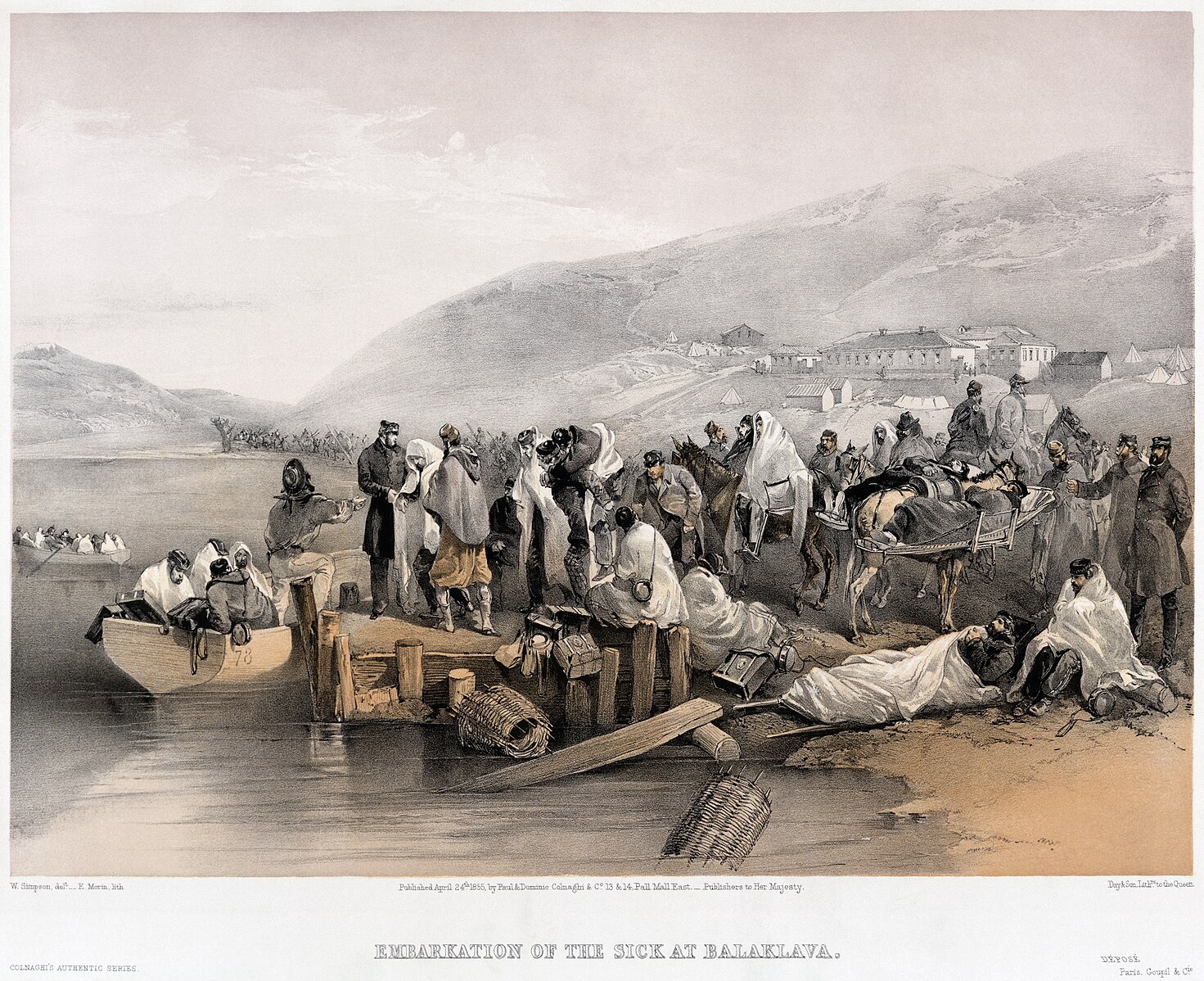
John Snow’s investigation is a classic case study of attempting to establish causality. Snow was a medical doctor and observed an outbreak of cholera in London in 1854. At the time, cholera was common and could lead to thousands of fatalities in a given wave.

It was not yet known that germs cause disease; the leading theory was that “miasmas” were the main culprit. Miasmas manifested themselves as bad smells and were thought to be invisible poisonous particles arising out of decaying matter. Parts of London did smell very bad, especially in hot weather. To protect themselves against infection, those who could afford to held sweet-smelling things to their noses.

For several years, a doctor by the name of John Snow had been following the devastating waves of cholera that hit England from time to time. He made the following observations:

• The disease arrived suddenly and was almost immediately deadly: people died within a day or two of contracting it.
• The pattern of infection was curious: Snow noticed that while entire households were wiped out by cholera, the people in neighboring houses sometimes remained completely unaffected.
• The onset of the disease almost always involved vomiting and diarrhea.

These facts are not compatible with miasma theory, which required that people who got cholera were inhaling bad air. For one, it is hard to understand why people in a single household would be affected, but not their neighbors, who were surely breathing the same air. Plus, the digestive symptoms suggest the disease comes from something people are eating or drinking, rather than breathing. Finally, if it were miasma (which is everywhere, all the time), it is hard to understand why some people suddenly fell ill but others did not. Snow’s prime suspect was water contaminated by sewage.

1.1.2 Theory and hypotheses

We will define a theory as being a:

conjecture about the causes of some phenomena of interest

Here the phenomena of interest is infection and death from cholera. Snow’s conjecture is that it is caused by the drinking of contaminated water. The conjecture of miasma theory is that the infections and death are caused by “bad air” of some kind.

We will compare the merits of these particular theories momentarily. First, note that “good” theories generally have the following properties:

• they have observable implications. This means that they predict something specific about the world which we can check via data.
• they are falsifiable. This means that we can imagine some observations in the world that are not compatible with our theory, such that we would have reason to doubt that theory is correct.

Many “theories” we come across in the world lack one or both of these properties. For example, many “conspiracy theories” are not falsifiable (they are “unfalsifiable”). This means that any evidence we find that runs contrary to the theory can be immediately accommodated by the theory. For example, when shown there is no evidence of a conspiracy, someone in favor of a conspiracy theory might say that this simply demonstrates how thorough the conspiracy was (!).

Note that a theory cannot be “proved correct”. For one thing, “proving” implies you can produce a “proof”, but that is specific to statements that can be shown to be mathematically true for all time given the assumptions you make or axioms you state. An example would be proving that \(\pi\) is an irrational number (the decimal repeats forever). We can prove theorems (like Pythagoras’ Theorem), but not theories.

What we may be able to do, however, is show that one theory is better than another. Or rather, more specifically, show that it is less wrong, as no theory is perfect. In general, we like theories that can explain more variation than others, which essentially means that they can predict an outcome (e.g. who will die of cholera) more accurately. A trade-off we typically face here is that theories that explain more are often more complicated. That is, they have more moving parts or more variables we have to record before making a prediction. Generally, we prefer simpler theories. Indeed, there is a name for this idea: Occam’s Razor. This is a rule that says that if two theories have the same explanatory power, we should prefer the simpler one. But if they don’t have the same explanatory power, and the simpler one predicts less well, Occam’s Razor won’t help much. Ultimately then, we may need to trade off explanatory power for simplicity (sometimes called “parsimony”).

To return to Snow, his theory was that sewage contamination in drinking water was causing cholera infections. Some local people had mentioned to him that the source of this contaminated water might be a pump on Broad Street. This allowed Snow to form a hypothesis, which is a testable explanation. In particular for Snow this will be that:

if we compare people who did and did not drink the water from the pump (“treatment”), we should see differences in infection rates (“outcome”).

We will define these terms in more detail below, but first, let’s look at Snow’s initial evidence as regards this hypothesis.

1.1.3 Snow’s visualization

At the end of August 1854, cholera struck in the overcrowded Soho district of London. As the deaths mounted, Snow recorded them diligently, using a method that went on to become standard in the study of how diseases spread: he drew a map. On a street map of the district, he recorded the location of each death.

Here is Snow’s original map. Each black bar represents one death. When there are multiple deaths at the same address, the bars corresponding to those deaths are stacked on top of each other. The black discs mark the locations of water pumps. The map displays a striking revelation: the deaths are roughly clustered around the Broad Street pump.

Snow’s first cholera map

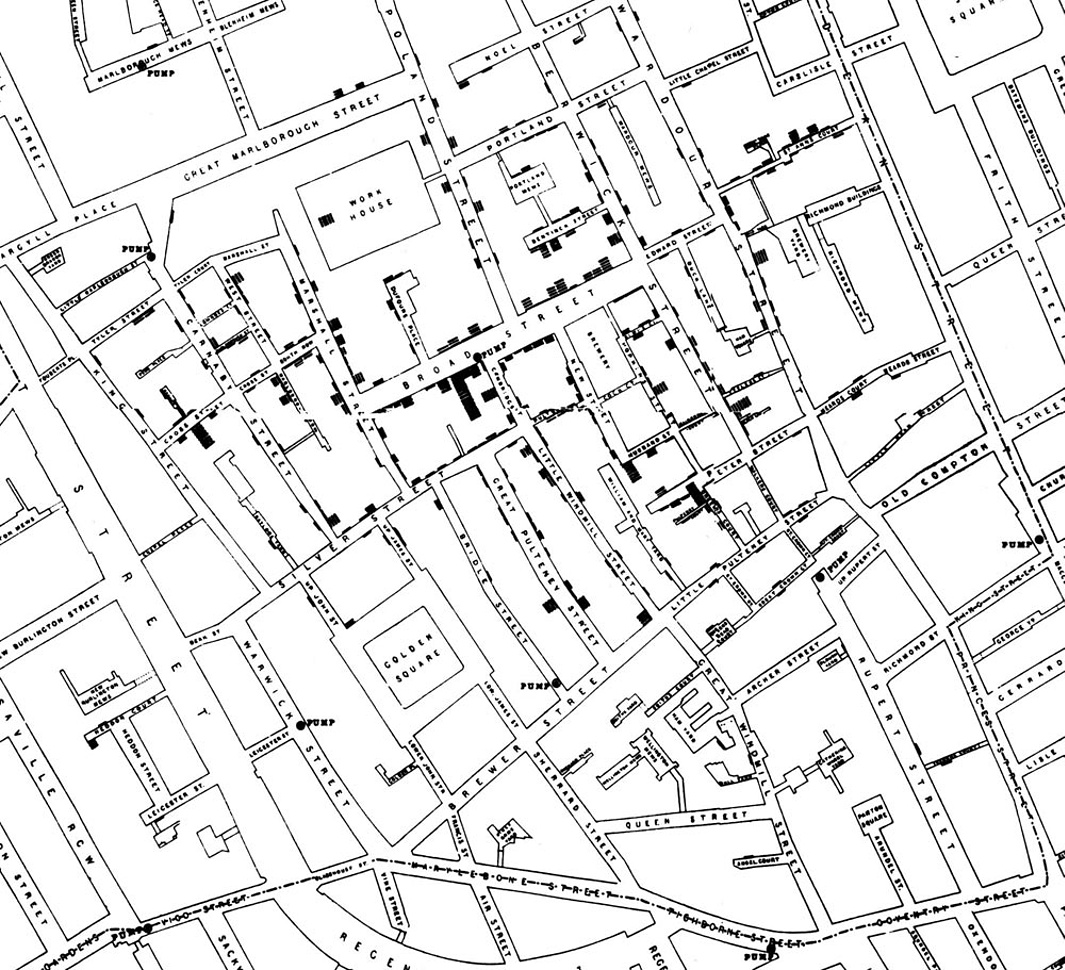
Notice, however, there are a few anomalies in the location of some of the deaths. Snow studied his map carefully and investigated the apparent anomalies. Even they, upon investigation, implicated the Broad Street pump. For example:

• There were deaths in houses that were nearer the Rupert Street pump than the Broad Street pump. Though the Rupert Street pump was closer as the crow flies, it was less convenient to get to because of dead ends and the layout of the streets. The residents in those houses used the Broad Street pump instead.
• There were no deaths in two blocks just east of the pump. That was the location of the Lion Brewery, where the workers drank what they brewed. If they wanted water, the brewery had its own well.
• There were scattered deaths in houses several blocks away from the Broad Street pump. Those were children who drank from the Broad Street pump on their way to school. The pump’s water was known to be cool and refreshing.

The final piece of evidence in support of Snow’s theory was provided by two isolated deaths in the leafy and genteel Hampstead area, quite far from Soho. Snow was puzzled by these until he learned that the deceased were Mrs. Susannah Eley, who had once lived in Broad Street, and her niece. Mrs. Eley had water from the Broad Street pump delivered to her in Hampstead every day. She liked its taste.

Later it was discovered that a cesspit that was just a few feet away from the well of the Broad Street pump had been leaking into the well. Thus the pump’s water was contaminated by sewage from the houses of cholera victims.

Snow used his map to convince local authorities to remove the handle of the Broad Street pump. Though the cholera epidemic was already on the wane when he did so, it is possible that the disabling of the pump prevented many deaths from future waves of the disease.

The removal of the Broad Street pump handle has become the stuff of legend. At the Centers for Disease Control (CDC) in Atlanta, when scientists look for simple answers to questions about epidemics, they sometimes ask each other, “Where is the handle to this pump?”

Snow’s map is one of the earliest and most powerful uses of data visualization. Disease maps of various kinds are now a standard tool for tracking epidemics.

1.1.4 Towards causality

The map gave Snow a strong indication that the cleanliness (or lack of cleanliness) of the water supply is associated with cholera. But he was still a long way from a convincing scientific argument that contaminated water was causing the spread of the disease. Indeed, this is what the science of epidemiology does: it works why a disease is spreading, and how to contain it.

In fact, this problem is very general: it is much easier to establish associations than it is to establish causation. The latter needs much more care.

1.2 Establishing causality is hard

Establishing causality is, in general, much harder than establishing associations (like correlations). Statements about causality rely on counterfactual reasoning. In particular, we will say that the

Causal effect of some factor \(X\) is the difference between what actually happened and what would have happened if \(X\) had been different in some way.

We can be even more specific. We can say that the

Causal effect of the treatment (\(X\)) on the outcome for a specific case at a specific time is the difference between the actual outcome and the hypothetical outcome that would have occurred, in the same case and at the same time, had \(X\) not been present.

The term treatment may remind you of medical trials, but it does not need to connote a drug specifically. The outcome could also be medical (e.g., got better or not), but need not be. For now, we will think of both the treatment and the outcome as being binary, meaning they take one of two values. That is, the entity under study either received the treatment or did not receive the treatment (and we will generally refer to the non-treated group as the control), and the outcome is one of two options. A case here will be whatever unit the causal effect (and the treatment) applies to: a patient, a resident of London, an animal, a country, etc.

In the case of cholera in 1854, an example of this reasoning would be:

the causal effect of drinking contaminated water (treatment) on infection status (outcome) for a particular person on a given day is the difference between their infection status after drinking the water and the infection status they would have had on the same day had they not drunk contaminated water.

As this example suggests, there is a Fundamental Problem of Causal Inference:

we never get to see both scenarios for the same unit (person) at the same time, and so we can never know the causal effect with certainty.

In other words, if I observe a particular person drinking from the pump on a particular day, I can record their outcome. But I cannot then go back in time and see what would have happened to that same person had they not drunk from the pump.

However, all is not lost. What we can do, and what Snow ultimately did, is find good comparison cases—some of whom receive treatment and some of whom do not (the control). Under some important conditions, we can compare those groups in terms of their outcomes and estimate the causal effect of treatment.

1.2.1 Experiments

Experiments allow us to estimate causal effects. We say estimate because, to reiterate, we will never know the effect with certainty owing to the Fundamental Problem of Causal Inference. The key components of an experiment are:

1. a treatment group and a control group, with a placebo
2. random assignment of treatment or control to subjects
3. double-blind design

Components (1) and (2) make the experiment a randomized control trial (RCT) (also called a randomized controlled trial). Component (3) is not technically required for an RCT, but it is preferred when possible.

In some cases, it may not be practical or ethical for an experiment to have all of these components. This does not mean we cannot learn anything about causation, but it does make the task more challenging. We will deal with each component in turn.

1.2.1.1 1. Treatment and control

The treatment group is:

the group of subjects (the units on which the experiment is being conducted) receiving the treatment.

The treatment could be almost anything: water from a pump, a leaflet to read, a job training program, or a life experience.

The control group is:

the group of subjects who do not receive the treatment.

Members of the control group may, however, receive a placebo, which is:

a pretend or “sham” treatment that the experimenter knows does not affect the outcome in and of itself.

A classic example in a medical trial is a sugar pill. It has no therapeutic value for curing the underlying disease being studied. Placebos help ensure that subjects do not know whether they are in the treatment or control group. This matters because simply believing one has received a treatment can affect reported outcomes. Our goal is to identify the real effect of the treatment, not the psychological effect of believing one has received it.

To calculate the causal effect of the treatment, we compare outcomes between the treatment and control groups. In practice, this often means accounting for a placebo effect, which is the effect that receiving the placebo has on outcomes reported by the control group.

A key observation here is that without a control group, causal inference is impossible. For example, Snow needs to observe people who did not drink contaminated water alongside those who did. Otherwise, he has no meaningful comparison. Similarly, in a drug trial, claiming that a treatment causes colds to improve after three days is uninformative without a control group, since many colds resolve naturally in that time.

For public policy questions, identifying a good control group can be especially difficult. Suppose we want to know the effect of a new state contraceptive policy on teen birth rates. A change in the birth rate may coincide with the policy, but could also be driven by other contemporaneous factors. Comparing to other states may help, but those states may differ in important ways.

Some problems are even harder. Consider asking what the effect of a particular U.S. President was on the economy. We do not observe a U.S. economy not governed by that President, making causal claims inherently difficult. In practice, we often try to construct as-if control groups, but doing so moves us away from the ideal experimental logic.

1.2.1.2 2. Random assignment

Suppose we are conducting an experiment for a new drug. Ideally, subjects should not select into treatment or control. By selection, we mean that subjects choose whether to receive the drug or the placebo. This is problematic because people who want the drug may differ systematically from those who do not—they may be sicker, more risk-tolerant, or otherwise distinct in ways that affect outcomes independently of the drug itself.

Random assignment solves this problem. For example, we might flip a coin for each subject: heads assigns them to treatment, tails to control. Randomization ensures that the treatment and control groups are the same on average, eliminating systematic differences that would otherwise bias causal estimates.

1.2.1.3 3. Double-blind design

Ideally, subjects should not know whether they are assigned to treatment or control. An experiment is single-blind if:

subjects do not know whether they are assigned to treatment or control.

Even better is a double-blind design, in which:

neither subjects nor the experimenter knows who is assigned to treatment or control.

This matters because experimenters may consciously or unconsciously treat subjects differently if they know group assignments, potentially biasing outcome measurement. Double-blind designs reduce this risk.

In practice, achieving double-blind conditions can be difficult. Consider surgical interventions such as bariatric surgery. Even with random assignment, it is hard to design a convincing placebo, since subjects will know whether they had surgery. Some studies attempt to address this using sham surgeries, but ethical and practical concerns remain.

1.2.2 Back to Snow

In Snow’s case, residents of Soho were not randomized into drinking from the Broad Street pump. Those who drank from it may have differed systematically from those who did not—for example, they may have been poorer or less healthy. As a result, Snow could not conduct a true randomized control trial.

Even if such a trial were feasible, it would not have been ethical. Assigning people to drink contaminated water would knowingly expose them to grave harm. This limitation is common in many important questions. We cannot ethically randomize people to smoke cigarettes for decades to study lung cancer. Instead, we rely on observational data, defined as:

data where the analyst does not control which units receive treatment and which do not.

In many observational studies, the analyst may not even fully understand how treatment came to be assigned.

1.3 Observational studies

To recap: Snow cannot pursue a randomized control trial. Instead, he must rely on observational data, which is a very common scenario. How, then, can he test his theory?

One key observation Snow made was that different areas of London were served by different water companies. In particular, some households received water from the Lambeth company, while others were supplied by the Southwark and Vauxhall (S&V) company. The former drew water from the Thames upstream of major sewage discharge, while the latter did not, and their water was often contaminated with sewage. The map below shows how these companies divided water supply across London residents.

Snow’s second cholera map

Snow showed that households supplied by the S&V company had cholera rates almost ten times higher than those supplied by Lambeth:

Supply Area	Number of houses	Cholera deaths	Deaths per 10,000 houses
S&V	40,046	1,263	315
Lambeth	26,107	98	37
Rest of London	256,423	1,422	59

Importantly, Snow argued that in the area of study, households did not differ in other relevant factors—such as income or baseline health—that might independently affect cholera rates. Notice what Snow is claiming: that the two groups differ only in terms of the treatment. One group (the treated) receives contaminated water, and the other group (the control) does not.

Snow could not randomize households to treatment or control. Instead, he argued that assignment via water companies was either as if random, or at least unrelated to other factors (such as wealth) that might affect the outcome (illness or death).

1.3.1 Snow’s legacy

In the short term, Snow was successful in persuading local authorities to keep the Broad Street pump handle removed, thereby saving lives. In the long term, his study became a classic, and his methods are now widely taught. His theory of fecal–oral transmission of cholera through contaminated water was eventually refined and accepted.

In the medium term, however, Snow’s ideas faced considerable resistance, and his methods were not widely embraced during his lifetime.

1.3.2 Natural experiments

Today, research designs like Snow’s are often referred to as natural experiments. These occur when:

assignment to treatment is outside the control of the experimenter but is either as if random, or at least unrelated to other factors (confounders) that affect the outcome.

We use the term confounders to refer to factors that affect both:

• assignment to treatment (treatment vs. control status), and
  
• outcomes.

In observational studies, confounders are a constant threat. Researchers can sometimes show that treatment and control groups are similar on observed variables (such as income or health), but they may still differ on unobserved variables (such as political attitudes or risk preferences). These are known as unobserved confounders.

For example, there is evidence that people who own dogs (treatment) have better heart health (outcome) than those who do not. But it is easy to imagine confounders—such as how much people enjoy outdoor exercise or how much free time they have—that influence both dog ownership and heart health.

1.3.3 Vietnam draft lottery

A more modern example of a natural experiment comes from studies using the Vietnam Draft Lottery in the United States. The draft lottery conscripted young men for military service based on their birthdays.

Intuitively, this is similar to placing all days of the year in a hat, drawing them at random, and requiring men turning 19 on the selected dates to serve. While this is a simplification, it captures the core logic.

Why is this useful? Men born on adjacent days—say August 5 versus August 6—are unlikely to differ systematically in important ways. This allows researchers to treat draft eligibility as as if random. Those drafted form the treatment group, and those not drafted form the control group.

This design allows estimation of the causal effect of military service on outcomes such as income or health. A classic paper using this approach is:

Angrist, Joshua D. “Lifetime earnings and the Vietnam era draft lottery: Evidence from Social Security administrative records.” The American Economic Review (1990): 313–336.

Angrist finds that military service reduced later earnings by roughly 15 percent.

This approach yields much more credible causal estimates than simply comparing people who choose to serve in the military with those who do not, since the latter comparison is plagued by confounders such as pre-existing health, income, or patriotism.

1.3.4 Compliance and non-compliance

In any experiment—natural or laboratory—we would like units assigned to treatment to actually receive the treatment, and units assigned to control not to receive it. This is known as compliance. The opposite situation is non-compliance.

Non-compliance is easy to imagine. In Snow’s case, some households assigned to S&V water might have obtained drinking water from Lambeth pumps. In the Vietnam draft lottery, some draftees refused to serve. If non-compliers differ systematically from compliers, causal inference becomes more difficult.

1.3.5 Terminology and practice in observational studies

In observational studies, common terminology includes:

• the outcome of interest: the dependent variable or \(Y\)
  
• the treatment: the independent variable or \(X\)
  
• confounders: variables \(Z\) that affect both \(X\) and \(Y\)

If \(Z\) drives both treatment and outcome, the observed relationship between \(X\) and \(Y\) may be spurious, meaning it does not reflect a true causal effect.

1.3.6 Testing hypotheses

As in Snow’s study, to test hypotheses we must:

compare units with different values of the independent variable (treatment status) in terms of differences in their dependent variable (outcomes).

The independent variable must vary across units; if everyone is treated (or untreated), causal effects cannot be estimated. Likewise, there must be variation in outcomes.

1.3.7 Selecting on the dependent variable

To make causal inferences, we must avoid selecting on the dependent variable, which means:

studying only cases that share the same outcome and attempting to infer what caused it.

Examples include studies of only high achievers or only long-lived individuals. Such designs make it impossible to know whether the observed characteristics are causal, because we lack comparison cases with different outcomes.

1.3.8 Survivor bias

Survivor bias occurs when a study includes only units that survive a selection process. This leads to biased inference because the observed units are systematically different from those that did not survive.

A classic example is Wald’s bomber from World War II. Engineers observed where returning bombers were damaged and initially proposed reinforcing those areas. Wald pointed out that these planes survived those hits; therefore, armor should be added where returning planes were not hit, since damage there likely caused other planes not to return.

Wald’s bomber (hypothetical illustration)

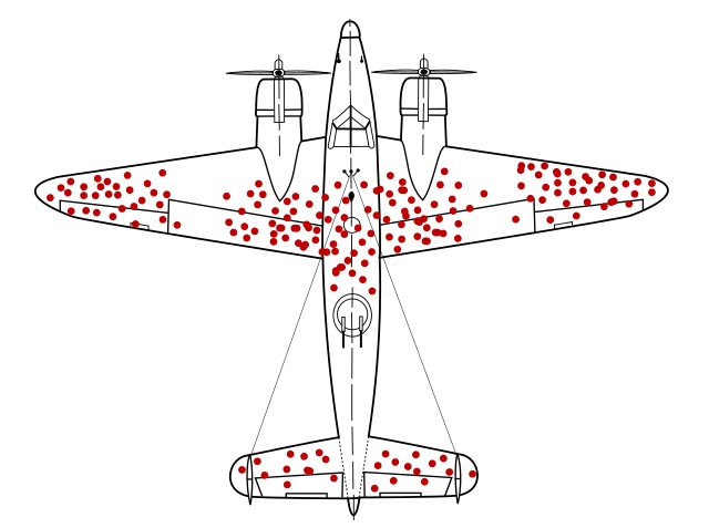
The key lesson is counter-intuitive but fundamental: to understand failure, we must consider the cases we do not observe.

1.4 More on causality

As we have seen, establishing that \(X\) causes \(Y\) is hard. Here we add to our discussion by introducing some basic principles to keep in mind when making a causal claim, along with terminology that is important to know in such circumstances.

1.4.1 General principles of causality

Establishing causal relationships typically requires that, at a minimum, we demonstrate:

1. covariation between the variables
2. temporal precedence: that treatment comes before outcome
3. we have controlled for third variables

We now briefly discuss each one.

1.4.1.1 1. Covariation

In general, we can objectively determine the association between two variables. Such measures include things like correlation, which we will cover later. If no association exists, this suggests that the variables do not covary, and it seems unlikely that \(X\) is causing \(Y\).

But this is not enough. For one thing, associations (e.g., correlations) do not imply causation: we can think of many situations where two variables are associated (like buying a dog and the owner’s heart health), but may not be causally related.

More difficult still, we sometimes have situations where a causal relationship exists but there is, in fact, no obvious association—at least in the data we have access to. For example, in the NBA (professional basketball association), height is not correlated with player performance or player value or player salary. These things do not covary with height. Studying only the NBA might lead us to believe height is unrelated to basketball ability in the broader world. But this is wrong, and due to a problem called conditioning on a collider, which is a more advanced topic.

1.4.1.2 2. Temporal precedence

In general, we want our treatment to precede our outcome: it is very hard to make claims about causality without this. But of course, there are many examples of one event consistently coming before another with no causal relationship: roosters crow in the morning, but they are not causing the sun to rise.

More subtly, there is no evidence that vaccines cause autism, though certain vaccines may be administered just before children are typically diagnosed with autism.

1.4.1.3 3. Confounders and controls

As we said, confounders—factors that influence both treatment status and outcomes—are a constant threat. One way to reduce our concern is to randomize subjects into treatment and control (and hope they comply with their group assignment).

If we cannot randomize, we may be able to control for known confounders. Here, control means take into account, and essentially means we compare within levels of the confounder to see whether there is any relationship between treatment and outcome.

A classic example is the relationship between ice cream consumption and drowning deaths. Months with more ice cream eaten (treatment) are also months with more drowning deaths (outcome). But this is probably not causal: it seems likely that ambient weather or air temperature is a confounder, \(Z\). When temperature rises, people eat more ice cream and also swim more, which leads to more drowning deaths.

If we control for weather \(Z\), we are implicitly comparing days at the same temperature (say, 85 degrees) and asking whether, within that set, days with higher ice cream consumption also have more drowning deaths. This is almost certainly not the case, and we can conclude the relationship is not causal.

1.4.2 Causal terminology

When we talk about causality, it is helpful to use certain terms in a specific way. Below, we first discuss types of causality; second, we introduce a common problem in assessing causal relationships (endogeneity); third, we clarify logical conditions as they pertain to causal relations; and finally, we discuss causal mechanisms.

1.4.2.1 Deterministic and probabilistic causality

How should we think about causality in general—beyond the definition of a causal effect? There are two broad possibilities:

1. Deterministic causation: if \(X\) causes \(Y\), then \(X\) occurring implies \(Y\) occurs. This is how we might model certain physical laws, such as gravity.
2. Probabilistic causation: if \(X\) occurs, \(Y\) is more likely (or less likely) to occur.

Deterministic causation claims are relatively rare in social science, and mostly arise in logical systems—for example, rules specifying what must happen under certain constitutional conditions.

Some scholars argue that essentially all causation is deterministic but appears probabilistic to us. That is, there may be specific factors which we could, in principle, observe and incorporate into our models, but in practice we cannot observe them all. For example, whether a tossed coin comes up heads or tails appears random, but if we knew the initial conditions (toss force, spin, air pressure, etc.), we could predict the result with certainty.

1.4.2.2 Endogeneity

You will regularly hear analysts refer to the problem of endogeneity. This can mean many things, but in general it refers to the idea that an independent variable (often the treatment of interest) is associated with something not included in the model, and that omitted factor also affects the outcome.

In this course, we will think about endogeneity as a specific problem: when \(X\) causes \(Y\) and \(Y\) causes \(X\). This is sometimes called reciprocal causation.

Examples include:

• democracy and development: higher levels of democracy may promote economic growth (e.g., via stronger legal protections), but higher income may also promote democratic stability (e.g., by increasing support for the political system).
• stress and physical illness: stress can contribute to illness, but illness can also contribute to stress.

In these cases, it is not straightforward to separate cause and effect. We cannot simply label one variable the treatment and the other the outcome and then compare treated and untreated units.

1.4.2.3 Necessary and sufficient conditions

When discussing causal relationships, it is helpful to clarify whether a factor is necessary, sufficient, both, or neither for a given outcome.

If \(X\) is a necessary condition for \(Y\), then:

• if \(Y\), then \(X\)
• \(X\) is required for \(Y\); \(Y\) cannot occur without \(X\)
• every time you observe \(Y\), \(X\) must be present

If \(X\) is a sufficient condition for \(Y\), then:

• if \(X\), then \(Y\) (but \(Y\) can occur without \(X\))
• \(X\) is sufficient for \(Y\); nothing else is required
• every time \(X\) occurs, \(Y\) will occur

Examples:

• being a U.S. citizen is necessary but not sufficient to vote for president.
• birth in the U.S. is sufficient but not necessary to be a U.S. citizen.
• the date being July 4th is necessary and sufficient for it to be Independence Day (in the U.S.).
• having a U.S. passport is neither necessary nor sufficient to run for President of the United States.

1.4.2.4 Causal mechanisms

A causal mechanism is:

a sequence of processes leading from \(X\) (the treatment) to \(Y\) (the outcome)

We need some sense of a possible causal mechanism to know what we should test and how. In Snow’s case, he suspected that consuming contaminated water led to cholera. This allowed him to set up his natural experiment via the water companies. He suspected fecal–oral transmission, but he did not know the specific biological process.

Later, scientists (such as Filippo Pacini and Robert Koch) refined the mechanism by identifying the role of the cholera bacterium. Refining mechanisms improves our understanding of how to prevent disease spread.

1.5 Being More Formal About Inference

Whether we are talking about the relationship between pump water (\(X\)) and disease (\(Y\)), or ice cream (\(X\)) and drownings (\(Y\)), we will ultimately obtain an estimate of the causal effect of \(X\) on \(Y\).

To fix ideas, suppose Snow compares the average incidence of Cholera (the proportion of people who have it) among those who have access to the contaminated water versus those who have access to uncontaminated water. As we said, we can think of the type of water you have access to as being our “treatment” (\(X\)) and we want to know the causal effect of that treatment on our outcome \(Y\), which is disease incidence. To do this, he takes a sample of a few hundred homes in each of the areas: 115 homes from the area exposed to the contaminated water, and 423 homes from the area not exposed to the contaminated water.

Here are his results:

Supply Area	Sample	Cholera Infections	Rate of Infection
Contaminated	115	4	0.350
Clean	423	2	0.005

Snow compares the value of \(Y\) (disease incidence) for those for whom \(X=1\) (contaminated) relative to the value of \(Y\) for those whom \(X=0\) (uncontaminated). This is 0.350-0.005 = 0.345.

Is this 0.345 the causal effect of water access on disease? Well, it’s an estimate of that causal effect, and using the terminology in Bueno de Mesquito & Fowler, we can be more specific about its nature. Those authors note, generally, that we can write

\[ \text{Estimate} = \text{Estimand} + \text{Bias} + \text{Noise} \]

Let’s walk through the terms:

• Estimate this is, literally, the number we get from doing the analysis: the actual difference in the means or rates or whatever that we calculate. In the Snow case above, the difference in rates was 0.350-0.005 = 0.345. But this might not be the causal effect.
• Estimand this is what are trying to estimate: the “real” thing in the population that we are trying to learn about. Here this the “true causal effect of contaminated water on disease incidence” (or something similar).

The problem is that the estimate (thing we calculated) might not be identical to the estimand (thing we were aiming to calculate) for two reasons:

1. Bias: these are systematic factors that make our estimate differ to our estimand. Above, we gave some concerns—some potential confounders—for the relationship between water supply and cholera rates. For example, perhaps poorer people who are already in worse health are more likely to live in places that have contaminated water—maybe property there is cheaper or certain industries located there attract poorer people to work. But then it isn’t the water that’s increasing the cholera rate—or not only the water. It’s that people’s pre-existing but unobserved poor health is leading to drink bad water and sepearately it is leading them to get cholera. In the extreme, the bad water might have no effect at all, once we control for pre-existing bad health. In that case, we are systematically deviating from the estimand of the causal effect of water on cholera when we produce our estimate in the way Snow did.

2. Noise: these are random factors that make our estimate differ to our estimand. For our purposes, this will mostly arise from the process of sampling. In the Snow case here, we said he is taking a sample of houses and trying to draw an inference from those about all homes in London. As we will see in subsequent lectures, the random sample(s) we take may vary somewhat just by chance from each other, and from the “true” distribution of all homes in London. We have very good ways to quantify how such noise affects our estimates: we will talk about things like “standard errors” below. In particular, when we take larger and larger samples, we can reduce the noise and increase our “precision”. Notice that, in the case of the pre-existing poor health confounder above, taking larger and larger samples mostly will not help our estimate approach our estimand: the bias remains, even if we can reduce the noise.

1.5.1 What if you have the “whole population”?

In Snow’s real work, he could potentially claim that he had the “whole population” of London, because he had the population level rates of access to various water supplies and their respective cholera rates. That is, he had all the data already: there is no other sample waiting to be taken.

Does that mean he doesn’t need to worry about noise? Put more specifically, and in a way that will become more obviously relevant in the next lectures, does this mean he doesn’t need to worry about standard errors (variance) on his estimates? Are those standard errors just zero, because he is not actually sampling?

A full answer here is technical, but in short: most statisticians would still want to see Snow think carefully about noise and communicating the nature of that variance around the estimate. This is because statisticians generally think about a given population (such as “London in 1854”) as being one hypothetical draw from a “superpopulation” of populations that could have been observed.

1.5.2 Potential Outcomes

Let’s return to Snow’s hypothetical samples above: he has 115 units (homes) who get treatment (bad water) and 423 who get control (uncontaminted water). We’ll say units for whom \(T=1\) are “treated” (get bad water) and those for whom \(T=0\) are “untreated”. Above, we used \(X\) for the treatment, but using \(T\) is a bit more intuitive for what follows. More generally, of course, “treatment” is an odd term for being exposed to something like an environmental hazard, but this literature developed from medical trials so we’re stuck with it.

Let’s think about a specific person or home or unit who could be exposed to the contaminated water, or could be untreated. We want to know what would happen to that person in terms of cholera if they got treatment versus if they were untreated. We will call them person \(i\) and think about the two scenarios—they get the treatment, or they don’t. Formally, we define

\[ Y_{\text{Treatment}=1, \text{unit}=i} \;\;\text{or}\;\; Y_{1,i} = \text{outcome for unit i if $T$ = 1} \] and

\[ Y_{\text{Treatment}=0, \text{unit}=i} \;\;\text{or}\;\; Y_{0,i} = \text{outcome for unit i if $T$ = 0} \]

Then the causal effect of being exposed to bad water is

\[ Y_{1i} - Y_{0i} \] The fundamental problem of causal inference tells us, however, that we can never observe this: that is, we cannot observe the same person \(i\) getting treatment and control at a particular time. They get treatment or control. Let’s suppose they got the treatment—that is, they live in a sewage affected area. In that case, we have an actual outcome for them (Cholera status) based on their treatment status (\(T=1\)). Ideally, we would know their potential outcome under control (\(T=0\))—that is, what would have happened had they not received treatment—and it would be a simple matter of comparing the actual outcome and the potential one. But, of course, this doesn’t work. Still, it provides a useful way to think about the problem.

Instead, let’s try to think about the effect for the whole population. That is, let’s think about the Cholera infection rate (the average) if everyone in London in 1854 had bad water and the average if they had uncontaminated water. We will define

\[\begin{align} \bar{Y_1} &=\text{ (average) infection rate if everyone in London had $T=1$ }\\ \bar{Y_0} &= \text{ (average) infection rate if everyone in London had $T=0$} \end{align}\]

1.5.3 Our Estimand: Average Treatment Effect

Here the “bar” notation just reminds us we’re talking about averages. We can define a new term now: the Average Treatment Effect. This is the difference between the average we would expect to see if everyone got treatment minus the average if no one got treatment:

\[ \text{ATE} = \bar{Y_1} - \bar{Y_0} \] We don’t ever get to observe this either, obviously: people in London either got treatment or control, and they didn’t get both. But we could try to estimate it. We cannot do much about the fundamental problem, but we could pretend we have access to everyone in the population and just compare those who got treatment (contaminated water) versus those who didn’t. We define:

\[\begin{align} \bar{Y}_{1T} &= \text{ (average) infection rate for everyone who had $T=1$ }\\ \bar{Y}_{0U} &= \text{(average) infection rate for everyone who had $T=0$} \end{align}\]

Then, the population difference in means is:

\[ \text{Population Difference in Means} = \bar{Y}_{1T} - \bar{Y}_{0U} \] In our example of Snow’s inference problem above, we thought about the situation where he had a sample of the population of interest, some of whom were treated (got contaminated water) and some of whom were not (had safe water). He could compare this treatment and control group to get the Sample Difference in Means:

\[ \text{Sample Difference in Means} = \underbrace{\bar{Y}_{1T} - \bar{Y}_{0U}}_{\text{population difference in means}} + \text{Noise} \] We have a noise term now, because we have random error induced by taking a sample rather than having the population itself.

1.5.4 Average Treatment Effect on the Treated

We now introduce another idea: the Average Treatment effect on the Treated (ATT). This takes the average of the hypothetical, unobservable effect of being exposed to the contaminated water supply among those citizens who were, indeed, exposed to it. It is defined as

\[ \text{ATT} = \bar{Y}_{1T} - \bar{Y}_{0T} \] This is the difference between the average rate of infection for those who had contaminated water minus what it would have been had this exact same set of Londoners not been exposed to that water, but instead lived in an area of safe water. As before, it’s a hypothetical: we don’t get to see what would have happened to these folks had they not got treatment, but it will be useful nonetheless.

Is our sample difference in means equal to this ATT (plus noise)? Maybe not. This is because, like we said, the folks that end up living in areas with sewer water may differ in important ways from those who live in areas of safe water. For example, they might be already poorer and sicker, such that their chances of getting cholera were much higher already.

In such a case, we would say that there are “baseline differences” between the Londoners who got the treatment and those who got the control. These are pre-existing (i.e. before the sewage was released into the water) and imply that even if we could measure the ATT, it wouldn’t be exactly equivalent to the difference in means that we observed.

How far off should we expect the ATT to be from the sample difference? It turns out that the bias is

\[ \text{Bias}_{\text{ATT}} = \bar{Y}_{0T}-\bar{Y}_{0U} \] This is the difference between the infection rate for those who were assigned to treatment (bad water) in the counter-factual world where they had received the control of uncontaminated water (\(\bar{Y}_{0T}\)) minus the actual average infection rate among the people who lived in the uncontaminated water area (\(\bar{Y}_{0U}\)) and got the control condition.

We have reason to believe this is not zero. In particular, it seems possible that even if the people who were exposed to sewage water had not received that water they would have higher cholera rates than the folks living in the clean water areas anyway. This is because, even without the sewage in their water, they were poorer and sicker to start with—and thus more susceptible to disease.

Just to put some real numbers on it, suppose that \(\bar{Y}_{0T}\)—the infection rate among people living in sewage water areas had they lived in “good” areas—was 0.01. And suppose that the infection rate among people living in “good” areas and not exposed to sewage water was 0.007. The first number is higher than the second, making the point that even if we hadn’t exposed the people who ended up getting sewage in their water, they still would have been more likely to get cholera. Now this wouldn’t be a problem if we had been able to randomize people to treatment and control: if we did that, we would expect no baseline differences, on average. That is, we wouldn’t expect the treatment or control group to start out being generally more susceptible to the disease, and we would find it easier to establish causal effects. Unfortunately, we can’t do that.

Back to the Sample Difference in Means. It can be written as:

\[ \text{Sample Difference in Means} = \text{ATT} + \text{Bias}_{\text{ATT}} + \text{Noise} \] Let’s suppose we have a very large sample (so the Noise term is essentially zero). And let’s think of the extreme case where the “true” ATT is also zero. That is, that the sewage water had no “extra” effect at all on the people who received it: they would have had exactly the same cholera rates, anyway, just from pre-existing bad health they already suffered from. Then it is possible that we could observe a Sample Difference in Means purely from the Bias term.

Put differently: there might be no causal effect of bad water, and all observed differences between treatment and control are driven by pre-existing baselines. Put differently still, we have:

\[ \text{Sample Difference in Means} = \text{ATE} + \text{Bias} + \text{Noise} \] This formula is a little complicated to calculate in practice because you have to take a weighted average of the ATT and the Average Effect of Treatment on the Untreated, but the main point is that you cannot generally interpret a difference as being equivalent to the ATE (the causal effect).

More basically still, \[ \text{Estimate} = \text{Estimand} + \text{Bias} + \text{Noise} \] which is how we began this section.

1.6 Being More Systematic About Bias

From Bueno de Mesquita and Fowler, we have our prevailing equation:

\[ \text{Estimate} = \text{Estimand} + \text{Bias} + \text{Noise} \]

This tells us that what we estimate (literally the difference in means, or proportions, or the correlation) as the relationship between treatment status (\(T=1\) or \(T=0\)) and the outcome might not be the true causal effect of treatment vs control. That causal effect we actually seek is the estimand. Unfortunately, this departs from what we calculated due to bias and noise. We will see how we can reduce noise later in the course—broadly, it involves increasing our sample size. But what about bias? Clearly, we would like it to be small, preferably zero. But can we say something more systematic than that?

Let’s return to our Snow example, and again suppose he compares a sample of treated units (received the contaminated water) with a sample of untreated ones (had clean water) in terms of their outcome (cholera rates). Suppose also that we think pre-existing poverty and ill-health is a plausible confounder. That is, we think that if you are poor, you are more likely to end up in an area with bad water, and more likely to get cholera anyway.

We think the causal diagram (where poverty is a confounder) looks something like this:

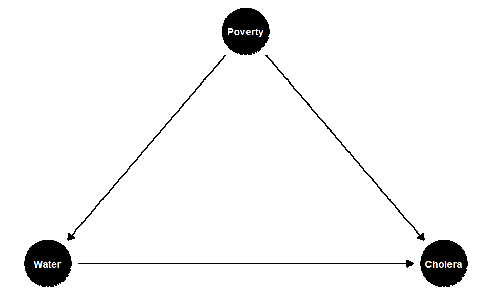
If the effect of poverty on your probability of treatment is positive, and the effect of poverty on your probability of the outcome is also positive, then poverty is pushing the correlation between the treatment and the outcome upwards. In the extreme, we cannot be sure that the treatment (the water) does anything to Cholera status—the true causal effect may in fact be zero. But if that’s true then not controlling for the confounder means we are overestimating the true causal effect by just looking at our estimated difference in means. This is a positive bias.

What if the confounder makes you less likely to get treatment and less likely to get the outcome? For example, suppose the confounder is “travel”. For instance, suppose that areas of London where the Thames is cleaner are easier to navigate by boat—there is less detritus in the water, it’s less unpleasant to be on etc. If you are the type of person who has to regularly use the river to go somewhere for work or leisure, you might select to live in areas where the water is less polluted. But if you travel a lot to outside of London, you are less likely to contract Cholera anyway (because you aren’t around Londoners who have it). So, you are less likely to get the treatment (bad water) and less likely to get the outcome (disease). But this causes the correlation between control (being untreated) and not getting the disease upwards, even though there is no new causal effect here. But this makes the control condition look “more effective” than it really is at preventing disease; and this will automatically make the treatment look more effective at giving you the disease. So this situation also means we are are overestimating the true causal effect by just looking at our estimated difference in means. This is thus also an example of a positive bias.

What if the confounder makes you less likely to be treated but more likely to get the outcome? In the Snow case, this would be a confounder that makes you less likely to have drunk the contaminated water from the Thames, but more likely to have cholera. One example might be British soldiers returning from Russia in the 1850s. There was a large outbreak of cholera in Russia at this time, so they were more likely to have it.

Embarkation of the sick at Balaklava (1855). Many of these men had cholera, presumably.

On the other hand, they were not exposed to the contaminated London river water necessarily (because they were away fighting), and thus are less likely to have received the Snow’s recorded treatment. So “being a British soldier” is a confounder that weakens the observed relationship between drinking London’s polluted water and having cholera. But this implies we are now under estimating the causal effect of bad water in London and the disease. In the limit, we could imagine having enough returning British soldiers in our sample that we end up thinking the relationship between drinking polluted Thames water (specifically) and getting cholera was zero. So this is a negative bias.

The final case if where a confounder makes you more likely to be treated, but less likely to get the outcome. It’s hard to think of something plausible along these lines for the Snow case, but perhaps something like “being a brewery worker” would qualify. That is, suppose that breweries are more common in areas with (historically) worse water. And suppose—as was the case in Soho—that people who work in breweries are more likely to have access to their own private wells. In that case, we would expect such workers to nominally be more exposed to the treatment—they live in areas where the pumps serve up sewage—but they are less likely to get sick because they don’t actually drink from them. Again, this will lead us to underestimate the causal effect of living in area where the water is polluted.

To summarize these points, see the table below:

Confounder	Effect on Treatment	Effect on Outcome	Resulting Bias
poverty	+	+	Positive
travel	−	−	Positive
military service	-	+	Negative
brewery worker	+	-	Negative

Notice that reverse causality is a special case of this discussion. Recall that the problem in reverse causality is that the outcome causes the treatment (at least in part). If the outcome has a positive effect on treatment, then it will look like the treatment is more effective than it really is: so this is a positive bias. If the outcome has a negative effect on treatment, it will look like the treatment is less effective than it really is: so this is a negative bias.

Why is any of this helpful? If one has the confounder of concern, the next step is just to control for it. We will see more on this in our discussion of regression. But even if you don’t have the confounder, “signing the bias” as the process as above is know, is helpful for thinking about how far off (and in what direction) your estimate is from your estimand (the true causal effect).

1.6.1 Confounders, Mediators and Mechanisms

Above, we talked about the nature of causal mechanisms and confounders. They are different ideas:

1.6.1.1 Confounder

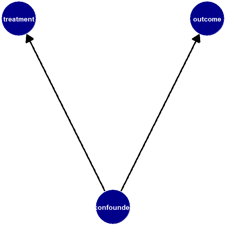
• a confounder affects the treatment and the outcome. A confounder is not affected by the treatment.
  
• We sometimes use the term pre-treatment covariate for confounders. This connotes the idea they come into play before treatment happens.

1.6.1.2 Mechanism

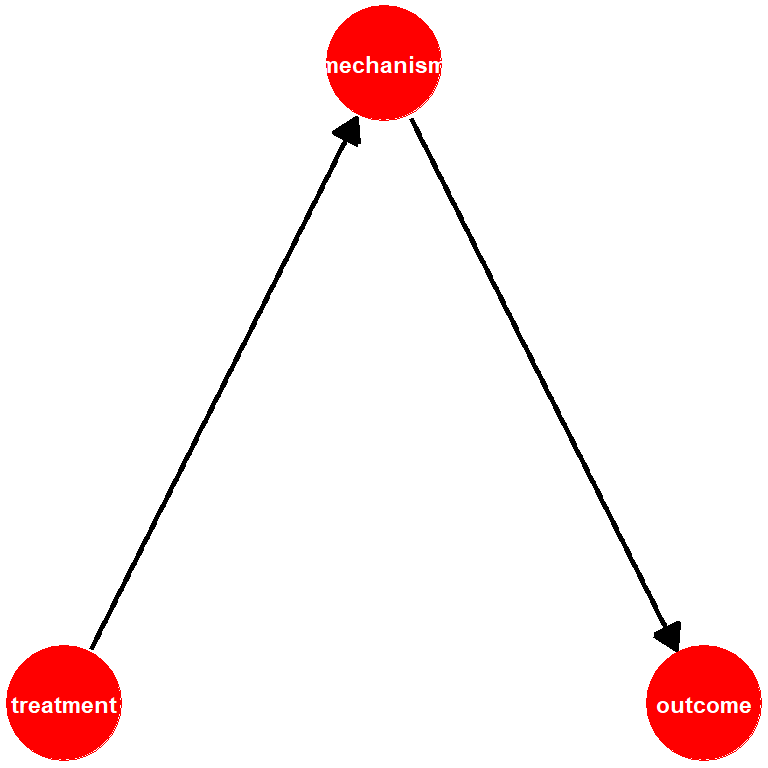
• a mechanism, also a mediator, is some feature of the data generating process that the treatment affects and it then goes on to affect the outcome.
• We sometimes use the term post-treatment covariate for mechanism. This connotes the idea that they come into play after treatment happens.

In many setups, the difference between these two ideas is clean-cut. For example, in the Snow case, we think poverty or pre-existing ill health is a good example of a confounder. This is plausibly pre treatment to living in certain areas and receiving sewage in your drinking water. Meanwhile, ingesting the relevant cholera bacteria from pump water seems a reasonable mechanism: it is post treatment to being served up sewage in your water, and would lead to you developing cholera. We don’t think people who have imbibed cholera bacteria are (for some reason) more likely to then drink from an infected pump (it doesn’t affect treatment). But in some cases, the difference can be confusing.

1.6.2 Education and Life Expectancy

To see why this can be confusing, let’s think public education, communicable disease rates and life expectancy. Take a look this graph of life-expectancy in England over the past two hundreds year or so—it’s from this article.

Life expectancy in England over time

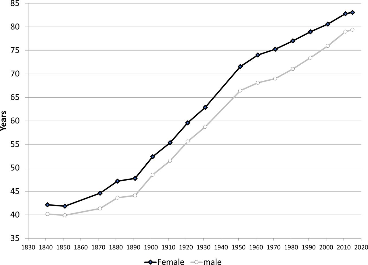
You can see that, in the late 19th Century, life expectancy increased more sharply than they had before. One theory might be that this is due to more widespread public education, which for young children was indeed made compulsory around 1870 in the UK. Suppose we notice a similar pattern across Europe: that is, more kids going to school regularly is positively correlated with people living longer.

Is this causal? Maybe. What should we do with other variables? For example, consider a variable like “rates of communicable diseases”. Suppose those rates decline at around the same time more education is introduced. Is that a mechanism, or a confounder? It seems one could argue it either way:

• it’s a mechanism insofar as a route by which more widespread education might lead to longer life expectancy is via telling people at school how they might avoid things like cholera—exactly the sort of thing Snow was interested in doing. So it’s post treatment to school.
• it’s a confounder insofar as we can imagine that changes in rates of disease cause uptake in education and longer life expectancy. It’s perhaps obvious how decreases in cholera mean people live longer, but we could also imagine as rates of disease decline, more kids go to school because they are healthier, not sick in bed, or helping parents who are too ill to work. In that case, it’s pre treatment to going to school.

In practice, we’d want to look at timing and perhaps find some unusual (natural) experiment setting to better identify a causal effect, but the main point here is that correlation and causation and very hard to tease apart in many cases.