6 Quasi Experiment

6.1 A Note on Interactions

Consider a new data set: this one is called world and has information on different countries.

world <- read.csv("data/world_data.csv")

6.1.1 Additive Models

A researcher has a theory about what determines the effectiveness of governments in different places. He thinks it depends in part on how educated a given population is: in particular, he suspects more educated people can hold governments to account better by reading newspapers, commenting online and so on. He measures this via the literacy (rate) of the country. He also thinks people in democracies probably have levers that make it easier to ensure government is effective: for example, bad politicians can be more easily replaced at elections. He includes a variable for that called `polity’ (Polity score) where higher numbers connote more democratic places.

He starts just by looking at correlations, and his results suggest this basic idea has support in the data: literacy and effectiveness are positively correlated; “democraticness” and effectiveness are also positively correlated.

cor(world$literacy, world$effectiveness, use = "complete.obs")

## [1] 0.5062999

cor(world$polity, world$effectiveness, use = "complete.obs")

## [1] 0.4003684

Then the researcher runs the following regression:

mod1 <-lm(effectiveness ~ literacy + polity, data=world)
summary(mod1)$coef

##              Estimate Std. Error   t value
## (Intercept) 2.2821589 6.77394855 0.3369023
## literacy    0.4765802 0.08250627 5.7762907
## polity      1.1765599 0.26985790 4.3599239
##                 Pr(>|t|)
## (Intercept) 7.367256e-01
## literacy    5.210885e-08
## polity      2.596470e-05

The coefficients on both variables (holding the other one constant) suggest increasing either increases how effective we think governments will be. So far so good.

As a theoretical matter, the analyst has put together an additive model of this form:

\[ Y = \beta_0 + \beta_1 X + \beta_2 Z + \varepsilon \] Here, \(X\) was literacy, \(Z\) was democraticness. An assumption underlying this model is that the effect of \(X\) is constant regardless of the value of \(Z\). Specifically that effect was 0.477. And vice versa: the effect of \(Z\) is constant regardless of the value of \(X\). Specifically, that effect was 1.17. To be explicit, if the democraticness of the country was 10 (approximately what it is for Australia), the effect of increasing literacy by one unit (1 percentage point) was to increase effectiveness by 0.477. Similarly, if the democraticness of the country was -10 (approximately what it is for Qatar), the effect of increasing literacy by one unit (1 percentage point) was to increase effectiveness by 0.477

More technically, we say that we are estimating parallel shifts in the outcome across the levels of \(X\) and \(Z\). We can see this more easily if we make these variable into binary (that is, zero or one) versions of themselves: we’ll use being above or below 90 as the cut point for literacy, and being above or below 9 as the cut point for democracy.

literacy2 <-  ifelse(is.na(world$literacy), NA, ifelse(world$literacy >= 90, 1, 0))
polity2 <- ifelse(is.na(world$polity), NA, ifelse(world$polity >= 9, 1, 0))

Now fit the regression again:

mod2 <-lm(effectiveness ~ literacy2 + polity2, data=world)
summary(mod2)$coef

##              Estimate Std. Error   t value
## (Intercept) 32.984262   2.129727 15.487555
## literacy2    9.210441   3.459802  2.662130
## polity2     26.185754   3.710469  7.057263
##                 Pr(>|t|)
## (Intercept) 1.765117e-31
## literacy2   8.729977e-03
## polity2     8.663469e-11

So we see the terms are statistically significant again, and positive (as expected). To see the parallel point, look at what happens when we move from the (binary) literacy variable being 0 to 1, for different (values) of democratic-ness:

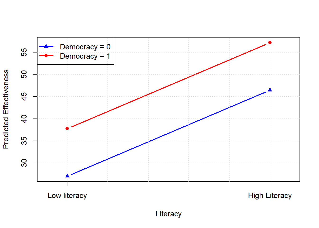
We see constant slopes and parallel lines: the intercepts differ, but the slopes do not.

6.1.2 Interaction Models

Suppose now that a new researcher thinks the effect of \(X\) is not simply constant and in addition to the effect of \(Z\). In particular, the she thinks the effect of \(X\) depends on the value of \(Z\), and the effect of \(Z\) depends on the value of \(X\). For example, she might think that for high literacy countries, increasing democraticness has a larger effect than for low literacy countries. So the effect is not constant.

Theoretically, this is a statement that we need an interaction term, which is a product of the two variables multiplied by each other, on which we place a new coefficient term \(\beta_3\)

\[ Y = \beta_0 + \beta_1 X + \beta_2 Z + \beta_3 (X \cdot Z) + \varepsilon \] This model estimates four mean (average) values, one for each combination of \(X\) and \(Z\):

\(X\)	\(Z\)	Expected \(Y\)	Interpretation
0	0	\(\beta_0\)	baseline: \(X\) and \(Z\) are zero
1	0	\(\beta_0 + \beta_1\)	Average Y when \(X=1\) and \(Z=0\)
0	1	\(\beta_0 + \beta_2\)	Average Y when \(Z=1\) and \(X=0\)
1	1	\(\beta_0 + \beta_1 + \beta_2 + \beta_3\)	Average Y when \(X=1\) and \(Z=1\)

In terms of how we interpret the coefficients, it is:

• \(\beta_1\): effect of \(X\) when \(Z = 0\)
• \(\beta_2\): effect of \(Z\) when \(X = 0\)
• \(\beta_3\): extra effect of \(X\) when \(Z = 1\) (or vice versa)

6.1.2.1 “Effectiveness” Example

We can be more concrete with our specific case: we’re modeling effectiveness based on literacy (\(X = 1\) for high literacy countries) and democraticness (\(Z = 1\) for high democracy countries):

\[ \text{Effectiveness} = \beta_0 + \beta_1 \cdot \text{Literacy2} + \beta_2 \cdot \text{Polity2} + \beta_3 \cdot (\text{Literacy2} \times \text{Polity2}) + \varepsilon \]

• \(\beta_1\): literacy gap among non-democracies
• \(\beta_2\): democracy premium among low literacy countries
• \(\beta_3\): how much more or less the democratic premium is for highly literate countries

Let’s fit the model and interpret the coefficients:

mod3 <-lm(effectiveness ~ literacy2*polity2, data=world)
summary(mod3)$coef

##                    Estimate Std. Error
## (Intercept)       34.830575   2.135825
## literacy2          3.353170   3.804176
## polity2            7.722616   6.754072
## literacy2:polity2 25.705144   7.969351
##                      t value     Pr(>|t|)
## (Intercept)       16.3077836 2.468138e-33
## literacy2          0.8814444 3.796917e-01
## polity2            1.1434014 2.549571e-01
## literacy2:polity2  3.2255002 1.588115e-03

Notice that, with lm, if you just use * on the right hand side, the model knows automatically to also include the non-interacted versions of the variables. That is, you would get completely equivalent results with

mod4 <-lm(effectiveness ~ literacy2 + polity2 + literacy2*polity2, data=world)

The model output (coefficients) are interpreted as:

• (Intercept): average effectiveness for low literacy non-democracies (34.83)
• Literacy2: difference in effectiveness when moving from low and high literacy among non-democracies (3.35)
• Polity2: difference in Effectiveness between non-democracy and democracy among low literacy places (7.72)
• Literacy2:Polity2: extra effect of more literacy among democracies (25.71)

In terms specifically of our interpretation of the interaction term:

• If positive, high literacy places get an extra boost from being democracies (as opposed to non-democracies).
• If positive, democracies get an extra boost from being high literacy.
  
• If negative, high literacy places get an extra reduction from being democracies
• If negative, democracies get an extra reduction from being high literacy (as opposed to low literacy)

In terms of averages, we have:

Literacy	Democracy	Expected Effectiveness	Interpretation	Example
0	0	\(34.83\)	baseline: low literacy, non-democracy	Angola
1	0	\(34.83 + 3.35 =38.18\)	Average Effectiveness for high literacy non-democracy	Vietnam
0	1	\(34.83 + 7.72 =42.55\)	Average Effectiveness for low literacy democracy	India
1	1	\(34.83 + 3.35 + 7.72 + 25.705 =71.60\)	Average Effectiveness for high literacy democracy	Australia

Clearly, there is an extra “bump” in effectiveness for democracy which are high literacy. In fact, looking at the regression table we see that only the interaction effect itself is statistically significant: the “main” effects, of literacy and democracy, are not (\(p>0.05\)). Taken literally, this implies there is

• no general effect of democracy on effectiveness
• no general effect of literacy on effectiveness
• there is an effect of the combination: that is, of being a high-literacy democracy (for example)

6.1.2.2 Visualizing the Interaction

It’s helpful to visualize the interaction, to make the point that, now, both the slopes and the intercepts will differ depending on the specific combination of variable values that a unit exhibits.

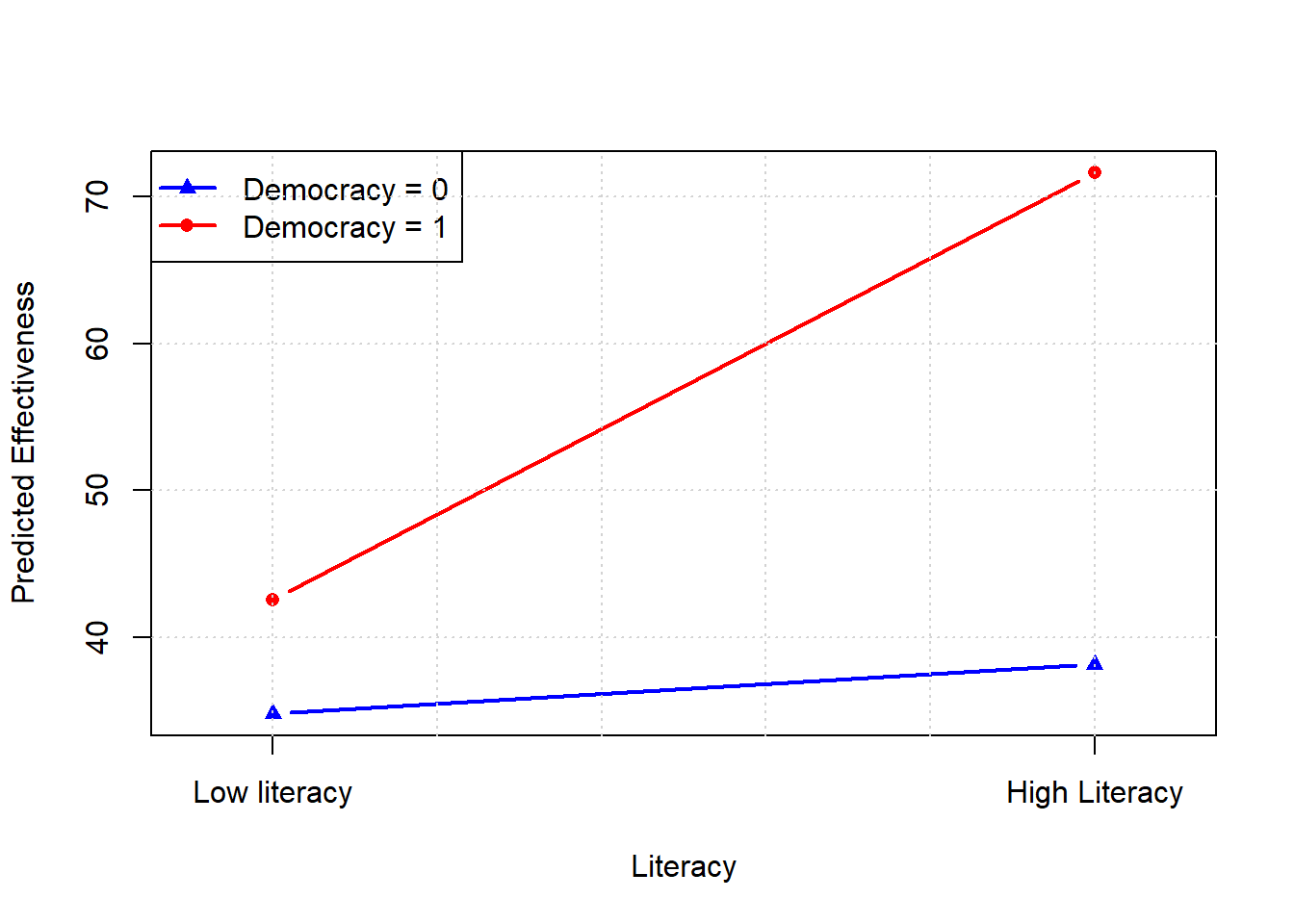
We see that the slopes are different, and so are the intercepts. Those intercepts are:

• for non-democracies: just the main intercept of \(\hat{\beta}_0 = 34.83\)
• for democracies: \(\hat{\beta}_0 + \hat{\beta}_2 = 42.55\)

The slopes are:

• for non-democracies: \(\frac{\Delta \text{Effectiveness}}{\Delta \text{Literacy}}\) when democracy \(=0\), which is \(\hat{\beta}_1 = 3.35\)
• for democracies: \(\frac{\Delta \text{Effectiveness}}{\Delta \text{Literacy}}\) when democracy \(=1\), which is \(\hat{\beta}_1 + \hat{\beta}_3 = 3.35 + 25.71 = 29.06.\)

6.1.2.3 Working with continuous predictors

The case where there were two variables—\(X\) and \(Z\)—and they took binary values (0/1) was particularly easy to conceptualize. But interaction models can cope with both variables being continuous, or one being continuous and one binary etc. Indeed, interaction models can also deal with triple (that is, three variable) or more interactions. In these cases, as you might expect, one needs more care with interpretation.

But just to see how it might work, let’s look at our original model with a continuous interaction:

mod_cont <-lm(effectiveness ~ literacy*polity, data=world)
summary(mod_cont)$coef

##                    Estimate Std. Error
## (Intercept)     23.60800848 8.40210161
## literacy         0.21202640 0.10312621
## polity          -4.58591530 1.48396697
## literacy:polity  0.06688063 0.01696481
##                   t value     Pr(>|t|)
## (Intercept)      2.809774 0.0057182269
## literacy         2.055989 0.0417695329
## polity          -3.090308 0.0024426826
## literacy:polity  3.942316 0.0001307131

As before:

• \(\hat{\beta}_1\) is the effect of literacy on effectiveness when polity is zero: 0.21
• \(\hat{\beta}_2\) is the effect of polity on effectiveness when literacy is zero: -4.59
• \(\hat{\beta}_3\) is how the effect of polity changes for a one-unit change in literacy, or how the effect of literacy changes for a one-unit change in polity.

What about the marginal effect of each variable? Well, holding polity fixed the change in effectiveness with respect to literacy is

\[ \frac{\Delta \text{Effectiveness}}{\Delta \text{Literacy}} = \beta_1+ \beta_3\text{polity} \]

So, it depends on the specific level of polity. Similarly, holding literacy fixed the change in effectiveness with respect to polity is

\[ \frac{\Delta \text{Effectiveness}}{\Delta \text{Polity}} = \beta_2+ \beta_3\text{literacy} \]

Immediately then, we see that in order to talk about the slope of the line, we need to specify at what values (of the other variable) we are assessing it. Some natural choice might be the maximum, the minimum and the mean. For example, here is effect of literacy on effectiveness, holding polity at these various values.

# Coefficients from model
b0 <- 23.60800848
b1 <- 0.21202640      # literacy
b2 <- -4.58591530     # polity
b3 <- 0.06688063      # interaction

# Range of literacy values: 0--100
literacy_vals <- seq(0, 100, length.out = 100)

# Choose three fixed levels of polity: min, mean, max
polity_vals <- c(-10, 4.38, 10)

# Create empty plot
plot(NA, xlim = range(literacy_vals), ylim = c(0, 100),
     xlab = "Literacy", ylab = "Predicted Effectiveness",
     main = "Effect of Literacy at Different Levels of Polity")

# Add prediction lines
cols <- c("blue", "black", "red")
ltys <- c(2, 1, 3)

for (i in 1:length(polity_vals)) {
  polity <- polity_vals[i]
  y_hat <- b0 + b1 * literacy_vals + b2 * polity + b3 * literacy_vals * polity
  
  lines(literacy_vals, y_hat, col = cols[i], lty = ltys[i], lwd = 2)
}

# Add legend
legend("topleft", legend = paste("Polity =", c("min","mean","max")),
       col = cols, lty = ltys, lwd = 2)
grid()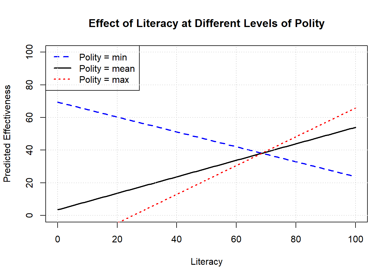

Notice that these lines have different slopes: the effect of increasing literacy is positive at he mean level of polity and at the maximum level. But it is negative at the minimum level of democracy: that is, the predicted effectiveness declines as literacy increases for those cases.

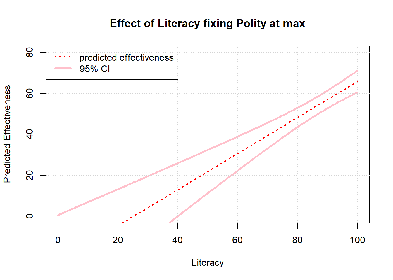
Of course, how confident we are in these effects is partly a product of how much data we have at the various values of interest. With that in mind, it might make sense to plot 95% confidence intervals on our predictions. Here we do that in the case of the maximum value of democracy, specifically:

6.2 Inference With Regression

6.2.1 When are Regression Coefficients Causal Estimates?

When can we treat our \(\hat{\beta}\) on the treatment variable as a causal effect of the treatment on the outcome? The answer is when some assumptions are met. That sounds strange but is true: if you are willing to believe certain assumptions about how your regression is set up relative to the world, you have a causal estimate. If you don’t believe those assumptions, you do not have a causal estimate. Consequently a lot of discussion in social science boils down to convincing people those assumptions hold. But ultimately, there is no definitive proof they do (or do not).

We’ll return to the assumptions momentarily, but for now think back to our regression of smoking rates on smoking taxes in the United States. Generically, we write such a regression like this:

\[ Y=\alpha + \beta X \] In the case of the using cigarette taxes to predict smoking rates in the various states, we can write it like this:

\[ \text{smoking rate}_i = \alpha + \beta\;\text{cigarette tax}_i+ \epsilon_i \] We use an \(i\) to denote the fact that we’re talking about the specific \(i\)’s state (say, New Jersey’s) values on the outcome variable (smoking) and treatment variable (the tax) and then we have a value of an “error term”, \(\epsilon_i\) which something random we cannot predict. Importantly, \(\alpha\), our estimate of the constant, and \(\beta\), our estimate of the slope, should not be indexed by \(i\)—we fit one for all units (states) in the data.

Here’s what we did, previously:

states_data <- read.csv("data/states_data.csv")
model <- lm(smokers12 ~ cig_tax12, data=states_data)
summary(model)

## 
## Call:
## lm(formula = smokers12 ~ cig_tax12, data = states_data)
## 
## Residuals:
##     Min      1Q  Median      3Q     Max 
## -9.6844 -1.7088  0.2418  2.4364  6.5657 
## 
## Coefficients:
##             Estimate Std. Error t value
## (Intercept)  23.3889     0.8385  27.895
## cig_tax12    -1.5909     0.4801  -3.314
##             Pr(>|t|)    
## (Intercept)  < 2e-16 ***
## cig_tax12    0.00176 ** 
## ---
## Signif. codes:  
## 0 '***' 0.001 '**' 0.01 '*' 0.05 '.' 0.1 ' ' 1
## 
## Residual standard error: 3.234 on 48 degrees of freedom
## Multiple R-squared:  0.1862, Adjusted R-squared:  0.1692 
## F-statistic: 10.98 on 1 and 48 DF,  p-value: 0.001756

Is the slope estimate, the \(\hat{\beta}=-1.59\) we obtained from ordinary least squares, the causal effect of the tax on the smoking rate? That is, is it the average treatment effect of \(X\) on \(Y\)? Well, that depends. In particular, it depends on some assumptions we may be more or less willing to make. For our purposes, the key assumptions will be:

1. Conditional Ignorability
2. Constant, homogeneous treatment effects
3. Correctly specified Model

We will discuss each in turn momentarily. For now note that one of the most important ideas is that we will need to control for confounders. We already met the idea of a confounder: it is a variable that affects both treatment status (including whether you got treatment or control, and how much) and outcome status (your value of \(Y\)). In the Snow case, we gave the example of pre-existing poverty: this may affect where you choose to live, and thus whether you have access to clean water. And it may also affect your pre-existing susceptibility to cholera. In the limit, we were concerned that people who are poor might end up exposed to bad water, and sick with cholera, but this wasn’t because sewage water causes cholera.

In the original cholera case, Snow made the point that he wasn’t too concerned about such pre-existing differences. He said

Each company supplies both rich and poor, both large houses and small; there is no difference either in the condition or occupation of the persons receiving the water of the different Companies…there is no difference whatever in the houses or the people receiving the supply of the two Water Companies, or in any of the physical conditions with which they are surrounded…

What if he had been concerned? Then he would have liked to have controlled for confounders like poverty. Controlling means “taking account of” the confounder you’re are worried about. In practice, in a regression context, it is about finding a way to look at the correlation between \(X\) and \(Y\) holding all other variables constant. In the Snow context, you can think of this as saying: “what’s the effect of water supply on disease rates in a world where all homes in all areas have the same level of pre-existing poverty and sickness (on average)?” That is, we find a way to adjust our understanding—the direction, the size—of the relationship between \(X\) and \(Y\) in light of something that might plausibly be leading us astray as to how they affect each other.

In our smoking example, what’s a plausible confounder? Education seems a concern. We could imagine that states with higher education levels smoke less anyway (they are more aware it hurts their personal health) and put more tax on cigarettes (perhaps more educated people think others should be discouraged from smoking due to knowledge of “second hand smoke” effects on kids). In the sample we have this is true insofar

• the correlation between smoking rate and proportion of citizens who finish high school (hs_or_more) is negative

cor(states_data$hs_or_more, states_data$smokers12)

## [1] -0.4929863

• the correlation between cigarette tax rate and proportion of citizens who finish high school is positive

cor(states_data$hs_or_more, states_data$cig_tax12)

## [1] 0.3043464

We control for this confounder by including it in our regression as a regressor—a “right hand side” variable.

model2 <- lm(smokers12 ~ cig_tax12 + hs_or_more, data=states_data)
summary(model2)

## 
## Call:
## lm(formula = smokers12 ~ cig_tax12 + hs_or_more, data = states_data)
## 
## Residuals:
##     Min      1Q  Median      3Q     Max 
## -9.3396 -1.6478  0.3278  1.3981  5.4290 
## 
## Coefficients:
##             Estimate Std. Error t value
## (Intercept)  58.7412    11.1410   5.273
## cig_tax12    -1.1437     0.4620  -2.475
## hs_or_more   -0.4145     0.1303  -3.181
##             Pr(>|t|)    
## (Intercept) 3.33e-06 ***
## cig_tax12     0.0170 *  
## hs_or_more    0.0026 ** 
## ---
## Signif. codes:  
## 0 '***' 0.001 '**' 0.01 '*' 0.05 '.' 0.1 ' ' 1
## 
## Residual standard error: 2.965 on 47 degrees of freedom
## Multiple R-squared:  0.3303, Adjusted R-squared:  0.3018 
## F-statistic: 11.59 on 2 and 47 DF,  p-value: 8.082e-05

We see immediately that the \(\hat{\beta}\) on our treatment has been reduced in magnitude: it went from \(-1.59\) to \(-1.14\). In absolute terms, the effect has been reduced by around 0.45. It is closer to zero than it was. This suggests that, before we were controlling for our confounder, we were saying the effect of cigarette taxes on smoking was more negative than it really was.

We will be more formal about this omitted variable bias in a moment. Before that, note that we don’t really care what value the coefficient (\(\hat{\gamma}\)) on the control took. This was not our estimand: our estimand was the causal effect of the treatment. Although some authors try to interpret these values, it is better (and less confusing) not to.

In terms of the omitted variable bias, Bueno de Mesquita and Fowler (p198–199) give a more complete derivation and we’ll summarize it here. For now, think about the regression we just ran as:

\[ Y = \alpha + \beta T + \gamma X + \epsilon \] Here, \(T\) is the treatment (cigarette tax) and \(X\) is a set of control variables. The coefficient on those control variables is \(\gamma\). We only have one control variable here—education—and our \(\hat{\gamma}\) was -1.14.

Compare this to our original regression:

\[ Y = \alpha^S + \beta^S T + \epsilon^S \] where we had no controls. We write \(\alpha^S\) and \(\beta^S\) here to remind us these the coefficients we get in the “short” version of the equation. In turns out that

\[ \text{Bias} = \beta^S - \beta = \pi\gamma \] Here, \(\pi\) is a measure of the correlation between control (education) and the treatment (cigarette tax): we noted that was positive. And \(\gamma\) is a measure of the correlation between the control (education) and the outcome (smoking rates): we noted that was negative. A positive multiplied by a negative is a negative, so we expect a negative bias overall. And that’s what we saw: naively estimating the regression as if there were no confounders led us to believe the effect of taxes on smoking was much more negative than it really was.

This logic is very general: if \(\pi\) and \(\gamma\) have the same sign, the implied omitted variable bias is positive (we say the treatment effect is too positive in the naive case); if they have different signs, the implied omitted variable bias is negative (we say the treatment effect is too negative in the naive case). Of course, both cases might imply the true treatment effect is closer to zero in absolute terms.

OK, so is our \(\hat{\beta}\) now the causal effect of the treatment on the outcome, given we have controlled for a confounder we were worried about? Well, let’s go through the assumptions we need to believe it is.

6.2.1.1 1. Conditional Ignorability

This means that we have controlled for all possible confounders. Another way to say this is that, given the regression equation and everything we are including in it, there are no other plausible baseline differences between the treatment and control groups that might affect their outcomes. Yet another way to say this is that, once we control for confounders, treatment is “as if randomly assigned” to the units.

In econometrics, this idea is sometimes called selection on observables—it says that, to the extent we can see (observe) a variable that we think might affect treatment and outcome status, we can put it in the regression and control for it.

Is that true here? Or could there be another confounder we would like to control for? Surely we can think of other things like “history of tobacco growing in the state”. We could well imagine that states that have grown tobacco historically would have more smoking and also lower taxes on cigarettes so as not to annoy tobacco farmers trying to sell their crops. There are many other such variables, such as “public health campaigns to improve lung health”. We can imagine people running such efforts would raise taxes on cigarettes, and also encourage people to quit smoking.

Determining the bias of missing some of these but not others is tricky. And these other confounders are ones we can actually observe and maybe record: there could be lots of variables that we cannot measure or control for.

6.2.1.2 2. Constant, homogeneous treatment effects

We need to be believe that the treatment effect is the same across all units: that is constant and homogenous. At least in our current set up, we cannot allow for a situation where, say, the effect of cigarette taxes on smoking rates in Kansas is much larger than the effect of cigarette taxes on smoking in Massachusetts. This is too bad, because we often believe such heterogeneous treatment effects exist.

A related problem is that when we add controls to a regression, we are implicitly re-weighting how certain observations (states in our case) contribute to producing the \(\hat{\beta}\). Specifically, adding controls means leaning more heavily on those units where treatment status is less predictable from the controls (units where the treatment status varies more given a specific value of the control variable). For us, that means we upweight states where their smoking rates are not as highly (perfectly) correlated with education levels.

This matters because it means that the coefficient estimate from our regression need not be the Average Treatment Effect but the Local Average Treatment Effect—where the term “local” refers to the idea that we are estimating the effect for those observations where we are plausibly varying the treatment status within a given band of values for the control. How large this the difference between the ATE and LATE actually is, and how much we should care about it, is a big area of debate.

6.2.1.3 3. Correctly specified Model

Finally, we need to believe some other things about our regression model. These are related to some of things we mentioned above in (1) and (2), but it’s helpful to be explicit:

• All relevant confounders included: we need to include them all, which can be hard both theoretically and empirically.
• No post treatment variables: we should not include variables whose values are determined occur after treatment. This messes up our estimates of the treatment effect from \(\hat{\beta}\). For instance, an obvious post-treatment variable for this problem would be “revenue generated from cigarette taxes”. This revenue variable will consume some of the effect that should “rightfully” belong to the tax level variable, and make it look less important in the data generating process than it really is. In this particular case, it seems relatively easy to identify such post-treatment problems and just leave out the variable. But suppose 25% of all cigarette tax revenue went to public anti-smoking campaigns. That variable is clearly post-treatment, but it’s also like a confounder insofar as we could imagine people running such campaigns set taxes in a way that allows them to afford such campaigns etc.
• correct functional form: we won’t press on this, but it’s plausibly the case that the relationship between cigarette taxes and smoking rates is non-linear. For example, perhaps cigarette taxes really matter when smoking rates are low, but not otherwise. This could cause problems for the exact causal effect interpretation.
• overlap/positivity: this is a technical requirement that says every unit—state in our case—could theoretically be treated or untreated, given their control variable values. Without it, we are in a world related to the heterogeneous effects problem above and we may not be able to obtain the ATE at all.
• no reverse causality: as usual, we need to believe \(X\) is causing \(Y\) and not the other way round.

6.2.2 Correlation becomes Causation via Assumptions

To reiterate, if we are willing to make certain assumptions, our correlations are causal estimates. Those assumptions may be more or less plausible, and more or less believable to different people. But they are just assumptions. Next, we will look at some techniques that people use when the “usual” assumptions to believe adjusted regression estimated are not very plausible.

6.3 Introduction to Quasi-Experiments

We are trying to estimate the causal effect of some treatment \(T\) or \(X\) on some outcome, \(Y\). We have explained that this is generally hard to do, partly because there are baseline differences between the treatment and control group that mean we cannot interpret any difference (or all the difference) in the outcomes for these groups as the causal effect. Specifically, we walked through this equation from Bueno de Mesquita and Fowler:

\[ \text{Estimate} = \text{Estimand} + \text{Bias} + \text{Noise}. \]

We said that one way to make sure there were no confounders—nothing causing both treatment status and outcome status—was to randomize treatment. But outside of experiments, that was hard to do. That is, we often have observational data where we don’t get to assign treatment, and we might not know who does assign it or how they do it. For example, here’s an infographic of the number of women in parliament in various countries:

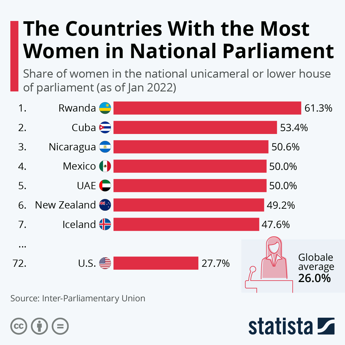
We might think this is a consequence of, say, the electoral system a country uses. But electoral systems are not randomized to units (countries), nor are they as if randomly assigned. So we said we would try to control for the factors—the confounders—that might be relevant. Still, this was hard: we often didn’t know all the confounders, or they were hard to measure.

Now we will talk about some techniques that will enable us to 1. help us tackle some difficult causal problems 2. enable us to make more plausible causal claims

These are called quasi-experiments because subjects are assigned to treatment/control in a way that is “as if” random, but not via explicit, deliberate, random assignment by the researcher.

6.3.1 Instrumental Variables

Above, we talked about the idea of reverse causality: this was a situation where a unit’s outcome affected their treatment status (i.e. whether they got treatment or control, or how much). This lead to bias: we thought the treatment was affecting the outcome, but it was actually (or in addition) that the outcome was affecting the treatment, which might then affect the outcome and so on. But then we were giving too much “credit” to the treatment for the effect we saw. “Instrumental variables” is the name of a technique for dealing with this problem: we (hopefully!) find a variable that isolates variation in the treatments in a way that’s as good as randomizing it, such that we can estimate the causal effect of treatment on outcome without concerns about reverse causality. It also can help with the more general situation where we think there are important omitted variables.

6.3.1.1 Endogeneity and Reverse Causality

In econometrics, we sometimes hear people say this sort of reverse causality leads to (or is an example of) endogeneity. The intuition behind this term is that there is something “in” the regression equation that we can’t observe and are not properly controlling for, that is affecting the causal inferences we are trying to draw. Technically, it’s defined as being opposed to exogeneity. This is an idea that comes from first writing out the regression equation like this:

\[ Y = \alpha + \beta T+ \epsilon \] where we would like to believe that \(\hat{\beta}\) (our estimate of \(\beta\)) is the causal effect of the treatment on the outcome. For this to be true, we need to believe that there’s nothing we are not controlling for that is causing \(X\) and \(Y\) (a confounder). We know there are things in the world that might be causing \(Y\) that we can’t observe: they are are in the error term \(\epsilon\). So we need to maintain that those things are not also causing \(T\) (treatment status). Technically we say we need the following equality to be true:

\[ \mathbb{E}[\epsilon|T]=0 \]

This says that, essentially, the value the other potential causal factors—things in the error term—takes doesn’t depend on someone’s treatment status. We call this exogeneity. When this is not zero, we have endogeneity. And a natural way this could happen is if \(Y\) causes \(T\). That is: \(T\) is now a function of \(Y\) and \(Y\) (as usual) is a function of \(T\) plus the error term. So this means \(T\) itself is a function of the error term (via being caused by \(Y\)). This induces a correlation between \(T\) and \(\epsilon\) and we say treatment status—or the “regressor”—is “endogenous”.

It’s not hard to think of examples of such systems:

• democracy and development: being a democracy might help countries economically, but then maybe becoming richer may help democracies stabilize, extend property rights and so on.
• smoking and ill-health: we think smoking hurts your lungs, but perhaps those who are sick are also more likely to smoke to relieve pressure.

In fact, the problem of endogeneity is very general, and it occurs anytime there’s something in the error term that we can’t control for that is affecting \(X\) (or \(T\)).

6.3.1.2 Charter Schools and Success

A popular example of a tricky causal inference problem is the effect of attending a charter school—a type of school that is funded by the government, but are mostly autonomous from local and state control. Economists, e.g. Angrist, Pathak and Walters, been interested in them for some time. Are these schools more effective than the usual “public school” alternatives? We might see their students do better on, say, standardized mathematics tests, but it’s hard to know if that’s because of the charter school or because the types of students who opt to go to charter school are systematically different in some important way from those that don’t.

That is, we might like to estimate a regression of this form:

\[ \text{math scores}_i = \alpha + \beta\;\text{attend charter school}_i+ \epsilon \] Where some people (some \(i\)) have the treatment (\(\text{attend charter school}==1\)) and some don’t. But it’s not hard to think of things (confounders) in the error term that might affect attending a charter school and your math score: for example, a supportive, pro-education family environment.

6.3.1.3 “As if” random assignment: Compliers and Non-compliers

How can we get out of this impasse? In general, it would be great if we could randomly assign a treatment like smoking or democracy or going to a charter school to the units. But this may be difficult or impossible. The instrumental variable approach instead seeks a variable \(Z\) such that the treatment is “as if” random for units. By “as if” we mean that \(Z\) is unrelated (uncorrelated) to other pre-existing factors that we would like to control for (e.g. family environment).

One great example of such a \(Z\)—an “instrument”—is a lottery. For instance, a lottery to go on The Hajj pilgrimage or to serve in Vietnam. Suppose that there is, indeed, a lottery for going to a charter school.

Straight off the bat, we need to think about two special groups who this lottery does not effect or at least not in the way we expect:

• first, there are some kids who do not go to the charter school (\(T=0\)), even though they ‘won’ the lottery to go (\(Z=1\)). They would have gone if they won, and if they didn’t, and we call them “always takers”.
• second, kids who did go to the charter school (\(T=1\)), even though they did not ‘win’ the lottery to go (\(Z=0\)). They would have not gone if they won, and if they didn’t win, and we call them “never takers”.

These groups are not “complying” with their lottery assignment, and we call them non-compliers. These groups mean that the lottery result does not perfectly determined treatment status. In general, we cannot learn much about Charter treatment effects from students who would always go to the Charter school or who would never go, whether they won the lottery or not. And we will rule out people—“defiers”—who do the exact opposite of their treatment assignment (go if they lose, don’t go if they win a place).

But we can learn from people for whom the lottery made the difference between whether they went to the charter school or not (subject to some other assumptions). These are the compliers (they do what their treatment assignment tells them to do) and we will compare those (randomly) in treatment and those (randomly) in control in terms of their math scores.

An important final point here is that we don’t actually need \(Z\) to be a lottery, specifically. It can be anything unrelated to pre-existing relevant \(X\)-variables—that is, stuff that affects treatment assignment and outcome. A classic example textbooks give is trying to determine the effect of smoking on health (as opposed to health on smoking). Suppose that some towns introduce a tax on cigarettes, and some do not. So long as we don’t think taxes affect health directly, then the tax \(Z\) is plausibly an instrument: that is, tax affects health only through reduces how much people smoke. So we may be able to calculate the causal effect by comparing the health outcomes of those towns that implemented a tax versus those that didn’t.

6.3.1.4 Assumptions

In keeping with the literature we will say:

• \(Y\) is the outcome. We will have it be continuous—like a math score.
• \(X\) (or \(T\)) is the treatment. We will have this be binary—like attending a charter school, or not.
• \(Z\) is the instrumental variable (the instrument), and it is binary—like “winning” the lottery (being sufficiently high in the lottery) or not.

For an instrumental variables (IV) approach to work, we need to make the following assumptions:

1. \(Z\) must have a causal effect on \(X\). This is the (strong) first stage requirement.
2. \(Z\) must not be correlated with other factors we would like to control for. That is, \(Z\) to be uncorrelated with the original error term in the original regression equation. We call this the independence assumption.
3. \(Z\) must affect \(Y\) only via the effect on \(X\). That is, to the extent \(Z\) changes the outcome, it must not do so directly—it must go via units allocation to the treatment (or not). This is the exclusion requirement.

6.3.1.5 Problems

In practice, it is very hard to find suitable instruments that satisfy all these requirements. Obvious violations include:

• weak instruments where \(Z\) doesn’t affect \(X\) very much (or at all).

Suppose, for example, that the smoking tax (\(Z\)) just doesn’t affect people’s consumption of cigarettes (\(X\))—they are all addicted and don’t care about price. In that case, the instrument isn’t affecting treatment status, whether or not treatment causes a big effect on outcomes. Weak instruments can be very misleading: the estimates we get can be even more biased than for a naive linear regression.

There is generally no “solution” to this problem, though one can at least look at how correlated \(Z\) and \(X\) actually are.

• invalid instruments (also “bad” instruments) where the \(Z\) is correlated with other things we should be controlling (violates independence) for and/or affects the outcome directly (violates the exclusion restriction).

In the charter school case, it could be that the same parts of a city or county that use lotteries for charter schools are also richer. In the extreme, suppose that poorer parts of the county don’t use lotteries at all (and send no one to charter schools). But now kids who are being allocated to charter schools by lottery in the county are already richer and potentially more likely to do well. This will make the charter schools look more efficacious than they really are.

Again, there isn’t much in the way of a “solution” here either, although one can check how “balanced” (how equal, essentially) those who win (\(Z=1\)) vs lose (\(Z=0\)) the lottery are on pre-treatment covariates. If it looks like winners are already much richer, we may have a problem.

We could obtain an exclusion restriction violation if doing well in the lottery affected math performance directly. For example, perhaps “winning” the lottery makes one feel more successful as a parent or student (even though it was random). That boost in confidence may help one do better on the math tests regardless of whether you go to a charter school.

There really isn’t much one can do to convince people the exclusion restriction holds. It mostly comes down to theory, though one can sometimes check whether \(Z\) affects other things it shouldn’t affect if the exclusion restriction truly holds.

6.3.2 Estimating IV

We’ll start this section with some data. In this dataset, we have

• score which is math achievement
• charter which is going to a charter school or not
• lottery which is getting lotteried into charter school consideration, or not.

Let’s load it, and start with the naive regression of math scores on charter attendance:

schooling <- read.csv("data/IVschooling.csv")
naive_model <- lm(score ~ charter, data=schooling)
summary(naive_model)

## 
## Call:
## lm(formula = score ~ charter, data = schooling)
## 
## Residuals:
##      Min       1Q   Median       3Q      Max 
## -2.76986 -0.68653 -0.00633  0.61983  3.02814 
## 
## Coefficients:
##             Estimate Std. Error t value
## (Intercept) -0.11664    0.04600  -2.536
## charter      3.48682    0.02275 153.277
##             Pr(>|t|)    
## (Intercept)   0.0115 *  
## charter       <2e-16 ***
## ---
## Signif. codes:  
## 0 '***' 0.001 '**' 0.01 '*' 0.05 '.' 0.1 ' ' 1
## 
## Residual standard error: 1.026 on 498 degrees of freedom
## Multiple R-squared:  0.9792, Adjusted R-squared:  0.9792 
## F-statistic: 2.349e+04 on 1 and 498 DF,  p-value: < 2.2e-16

This effect is positive as we would expect, but we worry about confounding. In this particular case, we know there was a lottery, but we can imagine some non-compliance: for example, richer students found a way to go to the charter anyway—even though they were not lotteried in.

We can get a sense of the non-compliance, just by comparing charter and lottery:

cor(schooling$charter, schooling$lottery)

## [1] 0.1098809

This is less than one, so it looks like the lottery doesn’t perfectly predict treatment. We need to try to incorporate the IV more systematically.

Traditionally, we estimate IV models using two-stage least squares (2SLS). The two stages are:

6.3.2.1 First Stage

Isolate the part of \(X\) (the treatment) caused by the instrument (\(Z\)). This is what we want to have in the regression of the outcome on the treatment. In practice, we fit this regression:

\[ X= \gamma_0+ \gamma_1Z + v \]

This is exactly what it looks like: we are regressing \(X\) (our treatment) as if its an outcome, on our instrument (\(Z\)) as if that’s the treatment in this equation. Here the \(\gamma\) are just coefficients, like \(\beta\)s. For every unit, we will now have a predicted \(X_i\), \(\hat{X}_i\). For our example:

stage1 <- lm(charter ~ lottery, data=schooling)
summary(stage1)$coef

##                Estimate Std. Error    t value
## (Intercept) -0.07129664  0.1234179 -0.5776848
## lottery      0.44412341  0.1800235  2.4670301
##               Pr(>|t|)
## (Intercept) 0.56373805
## lottery     0.01395931

X_hat <- fitted(stage1)

This last line makes the predictions for \(X_i\).

6.3.2.2 Second Stage

Take those \(\hat{X}_i\)s and put them in the second stage equation:

\[ Y = \alpha + \beta \hat{X} + \epsilon \] Even though \(X\) is endogenous, \(\hat{\beta}\)—called the instrumental variables estimate—from this equation is a good (technically, “consistent”) estimate of the causal effect of \(X\) on \(Y\). For our example:

stage2 <- lm(score ~ X_hat, data=schooling)
summary(stage2)$coef

##               Estimate Std. Error    t value
## (Intercept) -0.0309724  0.3732842 -0.0829727
## X_hat        2.8635073  1.4312270  2.0007360
##               Pr(>|t|)
## (Intercept) 0.93390659
## X_hat       0.04596316

This has reduced the coefficient size, but we are more confident we’ve captured the true causal effect because we are now relying only on the compliers: that is, the kids for whom the lottery made the difference. In fact, we can be more specific and say that the IV estimate reflects the treatment effect for compliers.

In practice one needs to do some corrections on the standard errors (the noise) to deal with the fact that the variable on the right hand side of the equation is estimated rather than fixed. But the principle is as we have done here.

6.4 Regression Discontinuity

In this part of the course, we are trying to find ways to “as if” randomize a treatment to units. Another way to put this is that we are trying to find a way to justify why a particular treatment assignment mechanism was as if random, such that we can make causal inferences. In the case of instrumental variables, we justified by saying that treatment was assigned by some variable \(Z\) that was “as good as” randomly assigned and that only influences the outcome via its affects on the treatment. This helped us avoid the problem of baseline differences, but such variables are very hard to find.

Now we look at a situation where treatment is determined via a cutoff rule: if you are “over” the threshold, you get treatment; if you are under the threshold, you get control. The idea is that people close to the threshold, it was “as if” random as to whether they were just over it or just under it, and thus those units are otherwise extremely similar. By “extremely similar” we mean they are (hopefully!) identical in terms of observed and unobserved characteristics and thus we can avoid the baseline differences problem. A closely related idea is that we need to believe that, at the threshold, nothing else changes. That is, we need to believe that for those who just got treatment (as opposed to just missed it, and got the control) the only thing different about their lives was being assigned treatment.

This approach will be called a Regression Discontinuity Design (RDD).

6.4.1 Background: the effects of a scholarship program

Suppose we are trying to estimate the effect of a special university scholarship program (treatment) on earnings after college. Perhaps the scholarship pays for some extra training, or networking, or generally just relieves financial burdens. Initially, we will suppose that the data we have is just all students’ outcomes (their salary) and whether they were in the special program or not. That regression looks like this:

scholars <- read.csv("data/scholarship_program.csv")
mod <-  lm(salary ~ scholarship, data=scholars)
summary(mod)$coef

##              Estimate Std. Error   t value
## (Intercept) 199507.52   637.7081 312.85086
## scholarship  46485.44  1147.2094  40.52045
##                  Pr(>|t|)
## (Intercept)  0.000000e+00
## scholarship 4.995335e-213

From this regression, it seems that getting the scholarship is worth an extra $46000 or so in salary. But it is plausible this is an overestimate: we can imagine that getting the scholarship is correlated with other things like being studious, or having family support, and that the true effect is a little lower. Supposing we had access to a confounder like family wealth, we might run the following regression:

mod2 <-  lm(salary ~ scholarship + family_wealth, data=scholars)
summary(mod2)$coef

##                   Estimate   Std. Error
## (Intercept)   1.641367e+05 7.014239e+02
## scholarship   2.629644e+04 6.661291e+02
## family_wealth 3.621625e-02 6.431927e-04
##                t value      Pr(>|t|)
## (Intercept)   234.0050  0.000000e+00
## scholarship    39.4765 5.513084e-206
## family_wealth  56.3070 6.373797e-312

This seems to reduce the effect of the scholarship a fair amount (down to $26000 or so), but it still may be too large if there are other confounders. Put starkly: it seems likely that smart or diligent or well supported students would probably earn more money anyway, even in the absence of a scholarship program.

6.4.2 Set up and general idea

Now suppose that to get into the scholarship program, there’s a hard cut off exam. Specifically, if a student gets 90% or more on the entrance test, they are assigned to receive the scholarship. If a student gets below 90% on the entrance test, they are not assigned to the program.

We can be a little more formal and write:

\[ \text{scholarship program} = \begin{cases} 1 & \text{if } \text{exam score} \geq 90 \\ 0 & \text{if } \text{exam score} < 90 \end{cases} \]

Suppose, in addition, that the following features hold:

1. treatment status is a deterministic consequence of the cut-off: if I know your score, I know your treatment. There is no probabilistic assignment here: we go from zero (no treatment, no scholarship) if you don’t hit the cut-off score, to getting treatment (scholarship) for sure if you do hit it. As an analyst, I don’t have to worry about who got the treatment: I know who did.

2. treatment status is discontinuous at the cut-off: your treatment status “jumps” at the threshold (0 to 1), but not before. You don’t get some scholarship if you almost hit the cut-off. You don’t get more scholarship if you hit 91 rather than 90. You hit the threshold or you don’t; you get it, or you don’t.

To these, we add another assumption called “continuity at the threshold”. This is a formal way of saying nothing, other than treatment status, changes when we are (just) above or below the cutoff. Taken together, these assumptions allow us to compare people (just) above and below the threshold, which means comparing people who got treatment versus those who got control. And from here we can make causal claims.

We can be more formal about these ideas by rewriting the equation above in a more general way:

\[ D_i = \begin{cases} 1 & \text{if } R_i\geq c \\ 0 & \text{if } R_i < c \end{cases} \] Here, \(D_i\) is the treatment status for unit \(i\), which you can also write as \(T_i\) or \(X_i\). And then \(c\) is the common cutoff (it is not indexed by \(i\)). \(R_i\) is the unit’s score, it goes by several other names in this literature:

• assignment variable: it decides your assignment to treatment or control
• running variable: units have a value that runs along this variable, and that determines their treatment status
• forcing variable: units have a value on this variable which forces them, deterministically, into treatment or control

6.4.3 The Inferential Problem and “Solution”

As we hinted, the basic idea is that around the 90% cutoff (i.e. a little above it and a little below it), those students who did not get into the program are very similar to those that did in terms of the observed and unobserved features they have—like home environment, studiousness and so on. From their perspective, getting into the scholarship program was as good as random. In fact, we could say it’s “exogenous”: the threshold was set prior to the students taking the test, and it cannot be changed by them (more on this in a minute).

6.4.3.1 Homogenous Slopes

All told then, the plan will be to compare the outcomes for those who just got it in, to those who only just didn’t make it, and draw causal conclusions. In order to make the causal comparison, in the simplest case, we need a regression of this form:

\[ \text{salary}_i = \alpha + \beta_1 \text{scholarship}_i + \beta_2\text{score}_i + \epsilon_i \] That is, a regression of the outcome on the treatment, but also the running variable (the exam score). Why do we need that latter piece? Well the idea is that we suspect there may still be a trend in which smarter/harder working students may get higher salaries, regardless of whether they were in the program or not. We’d want to check that there is some extra causal effect “bump” of the program over and above that effect.

Alternatively, we can dispense with what’s called the “smooth adjustment” for score if we just compare units very close to the cutoff with each other (above and below). In practice, this can be tricky because we perhaps do not have enough data (people) who are close enough to compare. So we do a controlled regression.

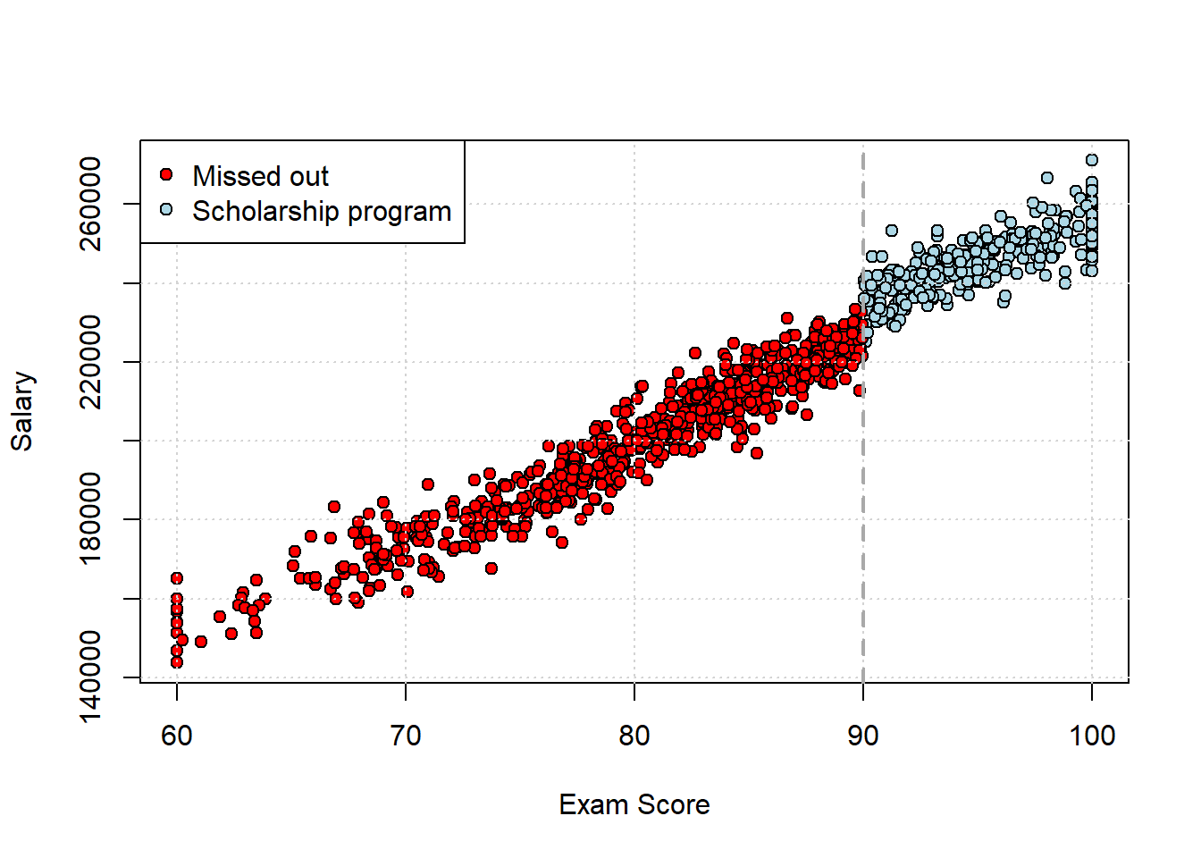
For our data, here is what the scatterplot looks like, with the threshold drawn on at the cutoff for the scholarship:

Let’s run the regression and draw lines on the plot for the fitted values it implies. We will also limit the data range a little to show the relationship in starker relief:

homog_mod <- lm(salary ~ scholarship + score, data= scholars)
summary(homog_mod)$coef

##              Estimate Std. Error   t value
## (Intercept) -4096.702  2175.5028 -1.883106
## scholarship  7440.820   553.2680 13.448854
## score        2546.778    27.0933 94.000289
##                 Pr(>|t|)
## (Intercept) 5.997695e-02
## scholarship 5.178174e-38
## score       0.000000e+00

homog_fit <- fitted(homog_mod) # fitted values

Straight off the bat, it looks like being in the program (vs not) does indeed matter: it’s worth around $7000 extra of salary, averaged over the whole sample. This is the Average Treatment Effect. In purple, we plot the fitted values for each person:

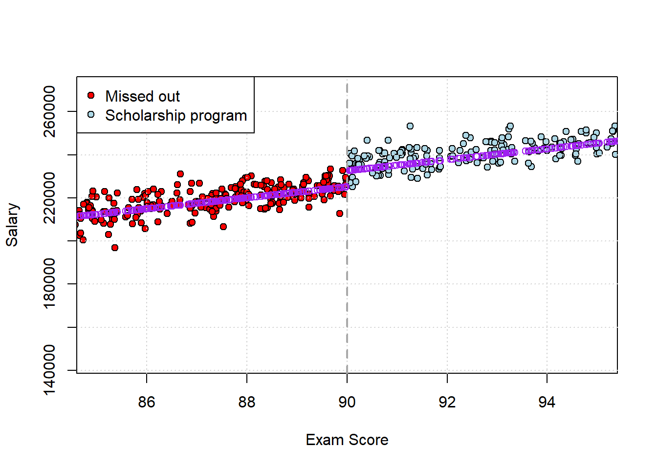
Clearly, there’s some sort of “step up” in salary (\(y\) axis) as we go from not being in the program (\(<90\) score) to getting in. Note that under very stringent assumptions, the $7000 effect of the program is the size of the jump at the threshold. But generally those assumptions—like slope homogeneity—are not completely met, and we’ll deal with that below.

6.4.3.2 “Bandwidth”

As we mentioned above, an alternative idea to estimate the effect is just to limit ourselves to units very close to the cutoff, and compare means. We have to select what is known as a “bandwidth”—how close to the threshold we want to look—to do this. Let’s select a wide and a narrow one, and compare the results.

narrow_data <- scholars[which(89 <scholars$score&scholars$score< 91), ]
narrow_dif <-t.test(salary ~ scholarship , data = narrow_data)$estimate

Here, the implied difference (for students scoring between 89 and 91) is about $11000. For the large bandwidth, we have

wide_data <-  scholars[which(60<scholars$score&scholars$score<100), ]
wide_dif <- t.test(salary ~ scholarship , data = wide_data)$estimate

Here, the implied difference (for students scoring between 60 and 100) is about $44000. These may both be too large (i.e. biased) for the reasons we discussed above. But clearly, when we take a wide window of points (the latter comparison) the bias is considerably worse because there is much more that varies between the students that we are not controlling for.

6.4.3.3 Heterogenous Slopes

The situation above was especially simple because we assumed the slopes were homogenous: that is, we assumed that the effect of the score was (linear and) constant (same slope) either side of the cut-off. This seemed reasonable from the plot: there is a “jump” at 90, but the slope of the lines is similar, but with an obviously different implied intercept. Another way to see this is just to estimate the same regression either side of the cutoff and compare the \(\hat{\beta}s\):

mod_below <- lm(scholars$salary[scholars$score<90] ~ scholars$score[scholars$score<90])
summary(mod_below)$coef

##                                      Estimate
## (Intercept)                         -9052.549
## scholars$score[scholars$score < 90]  2608.768
##                                     Std. Error
## (Intercept)                         2277.30297
## scholars$score[scholars$score < 90]   28.37272
##                                       t value
## (Intercept)                         -3.975118
## scholars$score[scholars$score < 90] 91.946334
##                                         Pr(>|t|)
## (Intercept)                         7.776855e-05
## scholars$score[scholars$score < 90] 0.000000e+00

mod_above <- lm(scholars$salary[scholars$score>90] ~ scholars$score[scholars$score>90])
summary(mod_above)$coef

##                                      Estimate
## (Intercept)                         60306.945
## scholars$score[scholars$score > 90]  1948.911
##                                     Std. Error
## (Intercept)                         7783.63147
## scholars$score[scholars$score > 90]   81.64183
##                                       t value
## (Intercept)                          7.747919
## scholars$score[scholars$score > 90] 23.871478
##                                         Pr(>|t|)
## (Intercept)                         1.374912e-13
## scholars$score[scholars$score > 90] 6.133999e-72

These slopes—2608.8 and 1948.9—are not identical but they are not too far off.

Often though, we need to allow for (very) different slopes on either side of the cutoff. For now we will assume everything is still linear, but we could imagine a situation where, say, students who get higher scores above the cutoff get disproportionately higher salaries later in life. Perhaps being the “best of the best” sets them up for other awards or improves their subsequent peer group. Alternatively, the story might be that for those qualifying for the program, doing better doesn’t matter—but it does matter for those who miss out. For instance, for the best performing ones there might be other scholarships or programs those folks are referred to by their professors, so they get some extra boost from doing better than otherwise. An example of such data is provided in the next snippet.

The key is that we need to add an interaction term to our regression model, in the way we need previously to allow for different slopes for different groups (here defined by treatment status):

\[ \text{salary}_i = \alpha + \beta_1 \text{scholarship}_i + \beta_2\text{score}_i + \beta_3(\text{scholarship}_i\times\text{score}_i) + \epsilon_i \] In R, we have

scholars2 <- read.csv("data/scholarship_program2.csv")
het_mod <- lm(salary ~ scholarship*score, data= scholars2)
summary(het_mod)$coef

##                     Estimate  Std. Error
## (Intercept)       -55351.477  2896.03309
## scholarship       118791.599 10522.94295
## score               2025.928    35.93775
## scholarship:score  -1036.282   111.66203
##                     t value      Pr(>|t|)
## (Intercept)       -19.11286  1.291459e-69
## scholarship        11.28882  6.788793e-28
## score              56.37327 3.652869e-312
## scholarship:score  -9.28052  1.022718e-19

We can see the interaction is significant, so we know that the effect of the scholarship now depends on the value of the student’s exam score. A good way to get a sense of the effects is to think about what happens to (average) salary when you from 80 to 90, versus 90 to 100.

new_data <- data.frame(
  score = c(80, 89, 91, 100),
  scholarship = c(0, 0, 1, 1)
)

predicted_salary <- predict(het_mod, newdata = new_data)

# Combine and label for clarity
new_data$predicted_salary <- round(predicted_salary)
new_data$group <- ifelse(new_data$scholarship == 1, "Scholarship", "Missed Out")

# Print results
print(new_data)

##   score scholarship predicted_salary
## 1    80           0           106723
## 2    89           0           124956
## 3    91           1           153498
## 4   100           1           162405
##         group
## 1  Missed Out
## 2  Missed Out
## 3 Scholarship
## 4 Scholarship

# assign outcomes to refer to in-text
below_boost <- new_data[2,3] - new_data[1,3]
above_boost <- new_data[4,3] - new_data[3,3]

so increasing your score by 9 points gets you about $18000 extra if you are below the cutoff, and (only) about $9000 more above. Let’s go back and plot the results in score salary space:

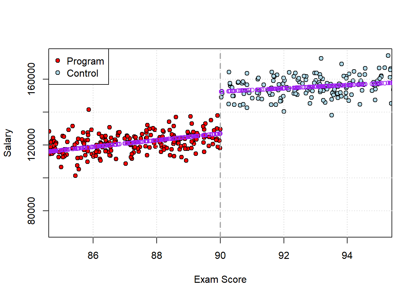And let’s just check the slopes in each part of the graph:

mod_below2 <- lm(scholars2$salary[scholars2$score<90] ~ scholars2$score[scholars2$score<90])
paste("slope below is", summary(mod_below2)$coef[2,1] )

## [1] "slope below is 2025.92834586977"

mod_above2 <- lm(scholars2$salary[scholars2$score>90] ~ scholars2$score[scholars2$score>90])
paste("slope above is", summary(mod_above2)$coef[2,1] )

## [1] "slope above is 989.646675551645"

As demonstrated by the regression, the effect of a higher score below the cutoff is larger than above: the slope is clearly steeper. Just a presentation matter, note that sometimes authors do the same regression but with centered data. Here, you subtract the cutoff (90) from the running variable (the score) and then run the regression. It becomes:

scholars2$score_centered <- scholars2$score - 90 # center
het_mod_center <- lm(salary ~ scholarship*score_centered, data= scholars2)
summary(het_mod_center)$coef

##                              Estimate
## (Intercept)                126982.074
## scholarship                 25526.249
## score_centered               2025.928
## scholarship:score_centered  -1036.282
##                            Std. Error
## (Intercept)                 422.42173
## scholarship                 807.90051
## score_centered               35.93775
## scholarship:score_centered  111.66203
##                              t value
## (Intercept)                300.60498
## scholarship                 31.59578
## score_centered              56.37327
## scholarship:score_centered  -9.28052
##                                 Pr(>|t|)
## (Intercept)                 0.000000e+00
## scholarship                2.458821e-152
## score_centered             3.652869e-312
## scholarship:score_centered  1.022718e-19

This tells us the scholarship is worth an extra $25526.25—this is the estimated discontinuity when one goes from below to above the threshold.

6.4.3.4 Local Average Treatment Effect (LATE)

Note that, because the slopes are heterogenous, we conclude that the treatment effect varies with score. But if that is true then what we are estimating is a Local Average Treatment Effect (LATE). It’s the average effect of the treatment at the threshold: that is, for those specific students who were close to the cutoff (on either side). We thinking about what would happen if those students who just got treatment instead got control, and vice versa.

Thus, this LATE is not necessarily telling us what the causal effect of winning the scholarship would have been for someone far from the cutoff, or generally not in close contention. The treatment effect for those students may be larger, smaller, or even be negative (they could be worse off). Formally, we say the causal effect for students not near the threshold is not identified by this design.

6.4.4 RDD in Political Science: Incumbency Advantage

The most common place you will see RDDs in political science is in estimating (party) incumbency advantage or incumbency bias. This is the idea that, once they win office, incumbents obtain some extra advantage that allows them to stay in office. For the US House, the re-election rate—essentially the proportion of incumbents who win if they seek to fight another election—is around 90%. We think this is true of individuals, but also parties. For instance, in a given US House Election, relatively few seats switch party control—just 17 of 435 in the 2024 cycle.

There are lots of theories as to why this incumbency advantage exists. For example, scholars argue incumbents find it easier to raise money. Or perhaps incumbents have better name-recognition among the public and media, and that helps their case. Finally, there are direct benefits that come with the job: for instance, incumbents have a “franking privilege” which essentially enables them to send mail to their constituents for free, thus allowing for credit claiming and publicity opportunities that challengers don’t have.

Whatever the reasons, obviously we would like to estimate how large or small this incumbency advantage is. One naive approach would be the following regression:

\[ \text{next election outcome}_i = \beta_0 + \beta_1 \text{incumbency status} + \epsilon_i \] where either the people running in the various districts are incumbents or they are not. But this won’t work very well, due to the usual problem of confounding. There are presumably lots of differences we can’t (easily) observe, like candidate or party “quality” or “charisma” that affect both treatment (incumbency) and outcome (winning or losing). In that case, our regression will over-attribute the causal effect to incumbency.

The central problem is that we cannot randomly assign incumbency status. But let’s think through how it would work if we could. For all the districts, we would:

• randomly assign a winning (and losing) party in some year, say 2012
• come back at the next election, say 2014, and see how much the winning parties do relative to the losing parties across all the districts

6.4.4.1 Close Winners and Losers

Because we randomized treatment (and control) this would give a good sense of how much incumbency matters for subsequent election performance. Of course, we cannot do this. But we can compare parties (candidates) that barely won (by, say, 0.5% of the vote) with those that barely lost (by 0.5%). The idea here is that election victory is as if (or as good as) randomly assigned to one party relative to another. The election was so close, that parties could not have known in advance whether they would win or lose, and they should look very similar on all the potential confounders we might be worried about.

As an example of such an election, consider Illinois’s 13th House District in 2012. The results were as follows—

Illinois 13th District, 2012

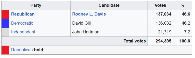
This was very close! The incumbent party, the Republicans, won by about a thousand votes and a very small percentage.

Suppose we found all such races that were similarly close, and treated winning as randomly assigned. This is an RDD in which:

• the running variable is the vote share or margin. We might define margin as, say, \(\text{Democratic vote share} - \text{Republican vote share}\).
• the threshold is coming top (or perhaps hitting 50% + 1 vote among the two big parties)

As “usual” we need to believe that

1. treatment status is a deterministic consequence of the cut-off: if I know your (relative) vote share (your margin), I know your treatment—whether your party won or not.

2. treatment status is discontinuous at the cut-off: your incumbency status “jumps” at the threshold (0 to 1), but not before. You don’t get some incumbency if you almost hit the top spot. You don’t get more incumbency if you get two votes over the threshold. You hit the threshold or you don’t; you get it, or you don’t.

And, of course, we need to believe that nothing else relevant to the outcome changes when treatment status does. Given what we wrote above, it won’t be too surprising to learn that analysts often fit a regression of the form

\[ \text{outcome next time}_i = \beta_0 + \beta_1 \text{incumbency status} + \beta_2 \text{margin}+ \beta_3 \text{incumbency status}\times\text{margin} + \epsilon_i \]

where the variables are:

• outcome next time: who won the next election? Democrats or Republicans? This is sometimes measured as probability of winning the next election
• incumbency status: this is the treatment of interest, and is allocated at the prior election
• margin: this a control for the running variable, to take care of the possibility that, even in some narrow bandwidth, there might be some extra bump up or down from being a bit more or less successful.
• interaction of incumbency status and margin: this takes care of potential heterogenous slopes that we mentioned above.

In practice, political scientists often restrict the sample to, say, cases where the parties are \(\pm 5\) percentage points away from each other (i.e. the closest margins). And they may also use certain automatic bandwidth selection methods combined with allowing non-linear effects near the cutoff—but that’s beyond the scope of this course.

6.4.4.2 Incumbency Bias in the United States

What is the magnitude of incumbency bias for the United States? Lee (2008) looked at the period 1946-1998, and found that parties that just win an election in a given seat are about 40% more likely to win subsequently in that seat relative to close losers. One of the main graphical results in that paper looks like this:

“Candidate’s probability of winning election \(t+1\), by margin of victory in election \(t\)” (from Lee 2008)

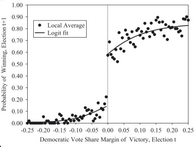
As you can see, at the threshold, just winning the election today (\(t\)) boosts re-election prospects by around 40 percentage points (\(y\)-axis) for next time (\(t+1\)). This corresponds to somewhere between 6 and 11 extra percent of the two party vote share.

6.4.5 What Could Possibly Go Wrong?

For RDD to identify the causal effect, we needed to make several assumptions. First, that treatment status is completely determined by the cutoff; second, that treatment status is discontinuous and “jumps” when the forcing variable hits the threshold. If we have reason to believe these do not hold, we have a problem. A major concern we might have is manipulation of the forcing variable. Our maintained assumption above was that units—other than via the running variable—could not consciously decide which side of the cutoff they would fall. But in real life we know that strategic actions from the units under study, or others, can indeed make these decisions not as if random. This issue is sometimes called sorting. And if units can “sort” around the threshold, then those just above may no longer be truly comparable to those just below.

For example, some students may cheat to make sure they just exceed the scholarship threshold (or professors may find ways to promote their preferred students to just over the cutoff), or politicians may strategically choose not to (re)run unless they think they will win. This would potentially lead to cases that “bunch” around the threshold (on either side)—whereas we should in fact observe a smooth distribution of the forcing variable. There are some ways to test for this.

Using simulated data, this is how it might look:

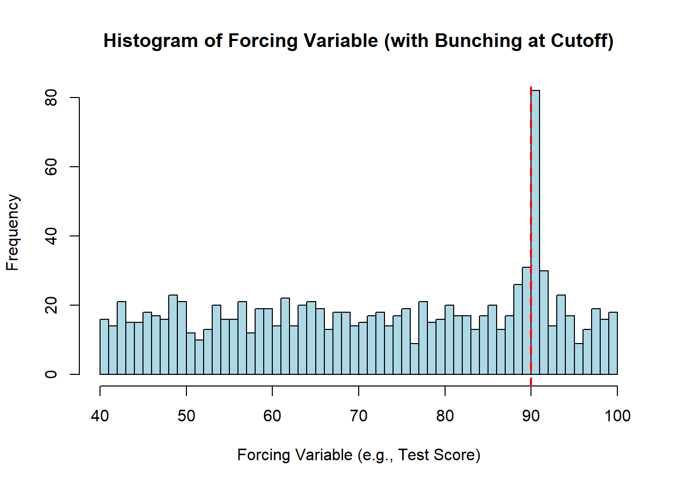
Notice how most test scores have an even or uniform number of students falling into that bin. But there is a large “bunching” at just over the key threshold for the scholarship—which might suggest students who would otherwise be in the bins just below the cutoff are finding ways to make sure they hit just above.

The other common issue is that something other than the forcing variable is affecting the outcome (and treatment status). That is, we want to believe that the units near the threshold are essentially identical except for the fact that some were just over the threshold, and some were just under. But if they differ in some other \(X\), this suggests they are not otherwise identical. This isn’t directly related to violations of deterministic assignment, but it may still be a problem. More formally, we describe this as discontinuities in the covariates. We can potentially ameliorate our concerns by looking at the students or congressional races near the threshold and check whether they are indeed “balanced” on the confounders we can observe (say, campaign funds raised). But we can’t do that for the variables we cannot observe.

In a 2011 paper, Caughey & Sekhon look at balance of winners and losers in US House elections on various covariates. This is their table:

“Covariate balance between treated (Democratic win: \(n\) = 43) and control (Democratic loss: \(n\) = 42) in a 0.5% window.” (from Caughey & Sekhon, 2011)

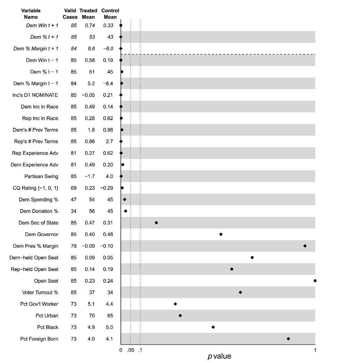
Variables near the top are unbalanced (the p-value for a difference in means is very low). This may or may not be a concern.

6.5 Difference-in-Differences (DiD)

To recap, we are trying to find ways to “as if” randomize a treatment to units. In the case of Regression Continuity, the idea was that there was an objective non-manipulable threshold and if you met that cutoff you got that treatment, and if you didn’t you were in the control condition. The key was that units who very close to threshold were (assumed) very similar in every other relevant way except their treatment status. So, in order to estimate the treatment effect, we simply had to compare those two groups.

== Now we look at a situation where treatment certainly isn’t random—indeed, units can opt into or out of treatment. But the key idea is that we will compare units who got treatment with units who got control, specifically in terms of how they changed over time using themselves as a baseline. That is, we will look at how the outcome changed for units who got treatment relative to their original outcomes and compare that to how the outcome changed for units who got control relative to their original outcomes. So long as the units were otherwise on similar, “parallel” trend paths in terms of those outcomes, this will identify a causal effect.

This approach will be called a Difference-in-Differences Design (DiD).

6.5.1 Background: NJ v PA fast food restaurants

The classic DiD example is from Card and Krueger (1994). They studied fast food restaurant labor markets in Pennsylvania and New Jersey, at a time when New Jersey raised its minimum wage, but Pennsylvania did not. The minimum wage level was the treatment. The outcome was unemployment. The authors measured that via the average number of employees in these restaurants before and after the change.

For New Jersey, the facts were as follows:

• February 1992: the average fast-food restaurant in NJ employed (\(Y\)) 20.44 people
• April 1992: New Jersey raised its minimum wage (\(D\)) from $4.25 to $5.05
• November 1992: the average fast-food restaurant in NJ employed 21.03 people (\(Y\))

Is this enough to conclude that increasing the minimum wage increased employment? Probably not, because we can imagine there may be other factors changing at the same time that changed employment. For instance, maybe the economy grew in general or maybe public taste for Big Macs increased. To try and identify the causal effect, Card and Krueger needed another, comparable state that did not have a minimum wage increase. They used Pennsylvania.

For Pennsylvania, the timeline was:

• February 1992: the average fast-food restaurant in PA employed (\(Y\)) 23.33 people
• April 1992: No change to minimum wage
• November 1992: the average fast-food restaurant in PA employed 21.17 people (\(Y\))

Can we just compare the situation in the states in November 1992, and conclude that the effect was \(Y_{NJ} - Y_{PA}=21.03-21.17 = -0.14\)? That is, can we conclude that the causal effect of New Jersey raising the minimum wage was -0.14 (less employment). Well, this would assume that New Jersey and Pennsylvania were otherwise completely identical. But we know there are lots of differences between the states that might affect employment at a given time: these might include income levels or tastes. So that won’t do.

6.5.2 Difference-in-Differences (DiD)

To recap: New Jersey was treated, Pennsylvania was not. The idea is then to:

• Measure the outcome in both before treatment (but only one is treated!)
• Measure the outcome in both after treatment (remember only one is treated!)

and then compare how each state changed relative to its baseline (value of outcome). This “difference-in-differences” tells us the effect of treatment. The actual data looked like this:

	NJ	PA	DiD
Feb 1992	20.44	23.33
Nov 1992	21.03	21.17
Change	+0.59	-2.16	2.75

At bottom right you can see the “difference-in-differences” was 2.75. This is calculated as:

\[ \begin{align} &= (\text{NJ in Nov} - \text{NJ in Feb}) - (\text{PA in Nov} - \text{PA in Feb}) \\ &= (21.03 - 20.44) - (21.17 - 23.33) \\ &= 0.59 - (-2.16) \\ &= 2.75 \end{align} \]

So, the effect of a higher minimum wage on employment was \(+2.75\).

Why does this work as a causal estimate? The idea—the assumption—is that whatever covariate or confounder differences there are between Pennsylvania and New Jersey, those systematic *differences are not changing over time**. If this is true, then any “extra” difference in November—over and above the difference in February—must be due only to the fact that New Jersey has been treated. In which case, if we subtract off the previous difference from the current difference, what’s left is the causal effect of treatment.

Note that, in principle, we could make sure we account for all relevant (non time varying) covariates with controls, explicitly. But that’s probably very hard to do in practice. So DiD is a good choice in that sense.

6.5.2.1 Parallel Trends

As hinted above, this requires the assumption of parallel trends. This assumption says that the change (not the level!) in the outcomes for the units would have been the same in the world where everyone was untreated. In terms of our example, we require that the change in employment levels for the states would have been the same had New Jersey never introduced a higher minimum wage. This does not require that the states start out or end up with the same specific levels of employment: it requires that the slopes of the lines along which the states moved are parallel to each other, wherever they start and finish.

Graphically, it requires a set up like this:

Implied DiD design from Card & Krueger

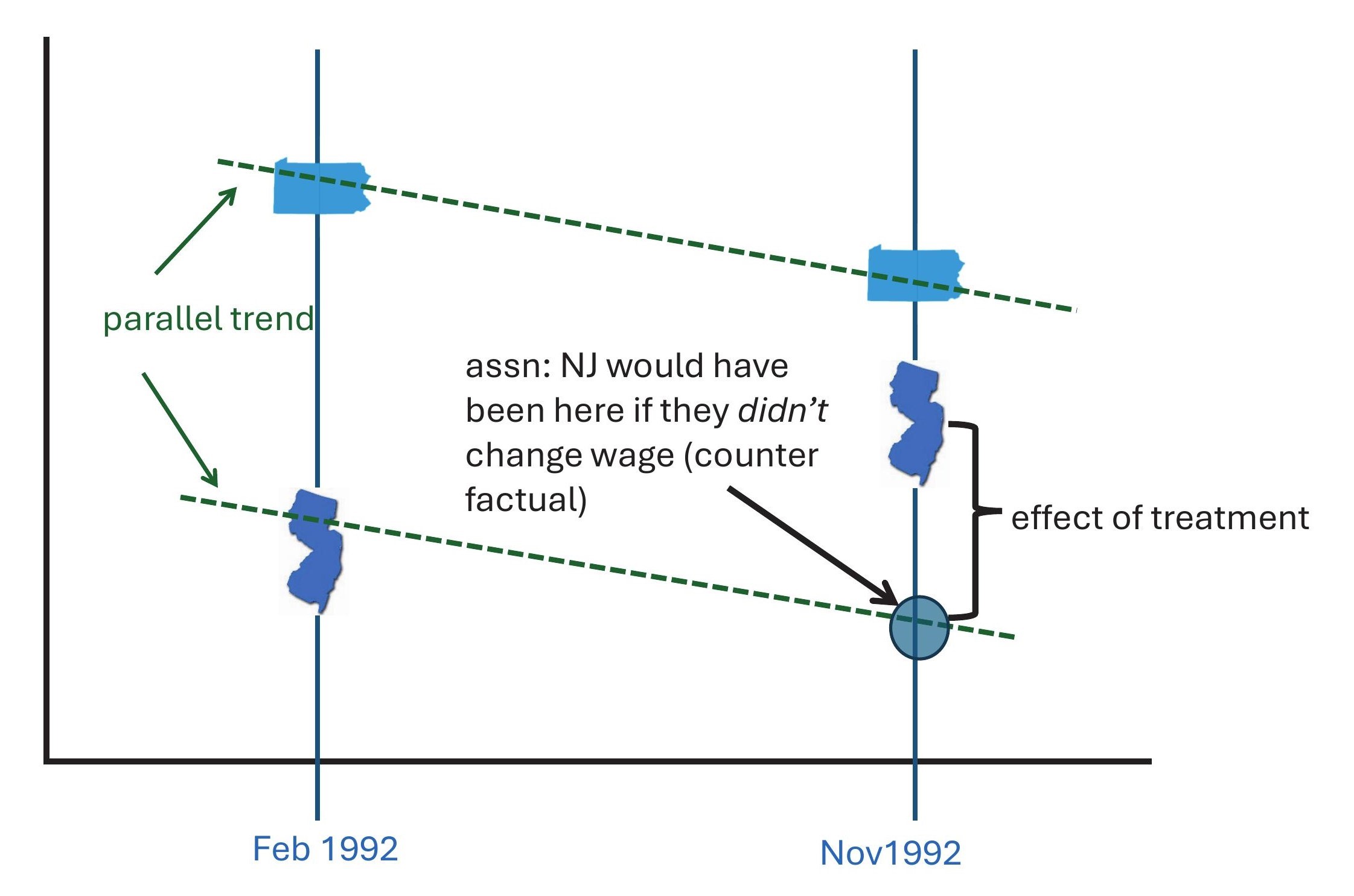
A nice feature of DiD designs is that they control for anything relevant that differs between the units but that does not vary over time. For example, in the case of New Jersey and Pennsylvania, their relative populations don’t vary much over the time period of this study: New Jersey had about 7.8 million people, Pennsylvania had about 12 million. This design controls for any effect on employment that this difference had.

6.5.2.2 What Could Go Wrong?

By contrast, DiD does not control for things that do vary over time. So we need to be concerned about any variable that potentially caused employment in New Jersey and Pennsylvania to evolve or change differently over time other than the minimum wage change. Suppose, for instance, that in response to New Jersey increasing the minimum wage, Pennsylvania cuts taxes on tips. Or suppose that New Jersey implemented the increase in minimum wage because it’s economy was (relative to other local ones) experiencing an upswing. These things would probably mean that even in the absence of treatment employment in New Jersey and Pennsylvania would not have followed similar trends over time.

What can we do about this? One idea is to check pre-trends. This is, we look at how employment changed over time before either unit was treated. Ideally, we would go back as far as we can historically, and check that those are parallel to each other: if they are diverging (or converging), this is likely a problem.

Another issue that is especially prevalent where the units being treated are geographically close is “spillovers”. As the wage rises in New Jersey, one can imagine that workers switch from restaurants in Pennsylvania and commute to New Jersey—especially in bordering areas. But now Pennsylvania is also getting treatment and this will typically drive down the difference between the states (and thus the causal effect) towards zero. This is a problem for parallel trends, and turns up as something called a SUTVA (Stable Unit Treatment Value Assumption) violation in the econometrics literature. SUTVA requires that one unit doesn’t “interfere” with another in treatment or outcome terms.

There is lots of recent work on problems and corrections for DiD designs. This includes extensions beyond the simple 2 unit \(\times\) 2 period case here: for example, we might have multiple units and multiple periods.